20. Writing Longer Programs#
20.1. Overview#
So far, we have explored the use of Jupyter Notebooks in writing and executing Python code.
While they are efficient and adaptable when working with short pieces of code, Notebooks are not the best choice for longer programs and scripts.
Jupyter Notebooks are well suited to interactive computing (i.e. data science workflows) and can help execute chunks of code one at a time.
Text files and scripts allow for long pieces of code to be written and executed in a single go.
We will explore the use of Python scripts as an alternative.
The Jupyter Lab and Visual Studio Code (VS Code) development environments are then introduced along with a primer on version control (Git).
In this lecture, you will learn to
work with Python scripts
set up various development environments
get started with GitHub
Note
Going forward, it is assumed that you have an Anaconda environment up and running.
You may want to create a new conda environment if you haven’t done so already.
20.2. Working with Python files#
Python files are used when writing long, reusable blocks of code - by convention, they have a .py suffix.
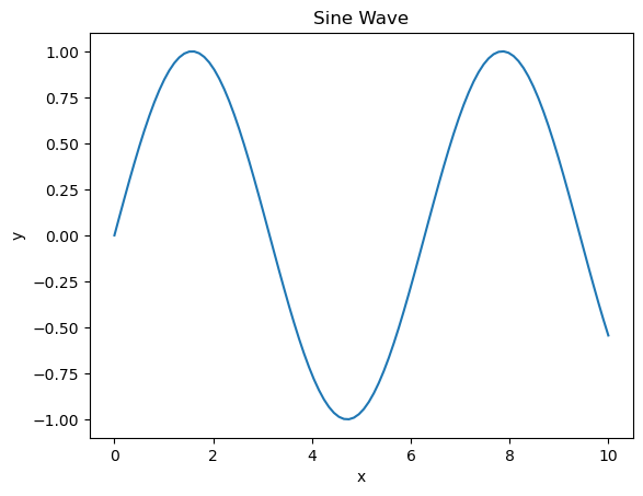
Let us begin by working with the following example.
import matplotlib.pyplot as plt
import numpy as np

x = np.linspace(0, 10, 100)
y = np.sin(x)

plt.plot(x, y)
plt.xlabel('x')
plt.ylabel('y')
plt.title('Sine Wave')
plt.show()
As there are various ways to execute the code, we will explore them in the context of different development environments.
One major advantage of using Python scripts lies in the fact that you can “import” functionality from other scripts into your current script or Jupyter Notebook.
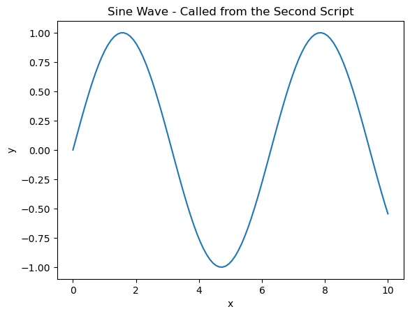
Let’s rewrite the earlier code into a function and write to to a file called sine_wave.py.
%%writefile sine_wave.py

import matplotlib.pyplot as plt
import numpy as np

# Define the plot_wave function.
def plot_wave(title : str = 'Sine Wave'):
  x = np.linspace(0, 10, 100)
  y = np.sin(x)

  plt.plot(x, y)
  plt.xlabel('x')
  plt.ylabel('y')
  plt.title(title)
  plt.show()
Writing sine_wave.py
import sine_wave # Import the sine_wave script

# Call the plot_wave function.
sine_wave.plot_wave("Sine Wave - Called from the Second Script")
This allows you to split your code into chunks and structure your codebase better.
Look into the use of modules and packages for more information on importing functionality.
20.3. Development environments#
A development environment is a one stop workspace where you can
edit and run your code
test and debug
manage project files
This lecture takes you through the workings of two development environments.
20.4. A step forward from Jupyter Notebooks: JupyterLab#
JupyterLab is a browser based development environment for Jupyter Notebooks, code scripts, and data files.
You can try JupyterLab in the browser if you want to test it out before installing it locally.
You can install JupyterLab using pip
> pip install jupyterlab
and launch it in the browser, similar to Jupyter Notebooks.
> jupyter-lab
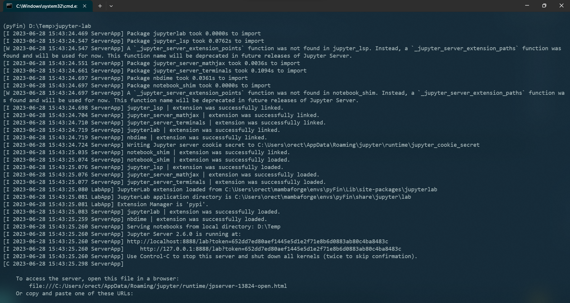
You can see that the Jupyter Server is running on port 8888 on the localhost.
The following interface should open up on your default browser automatically - if not, CTRL + Click the server URL.
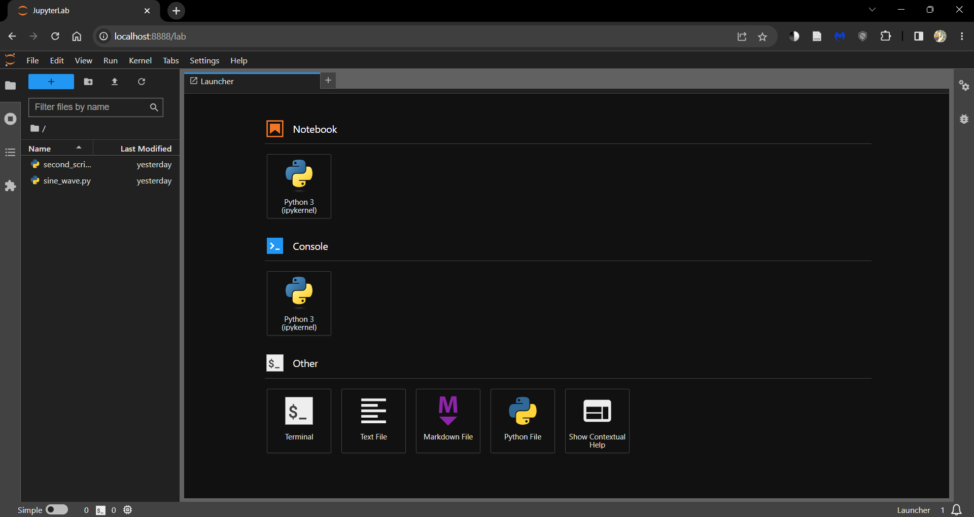
Click on
the Python 3 (ipykernel) button under Notebooks to open a new Jupyter Notebook
the Python File button to open a new Python script (.py)
You can always open this launcher tab by clicking the ‘+’ button on the top.
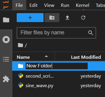
All the files and folders in your working directory can be found in the File Browser (tab on the left).
You can create new files and folders using the buttons available at the top of the File Browser tab.
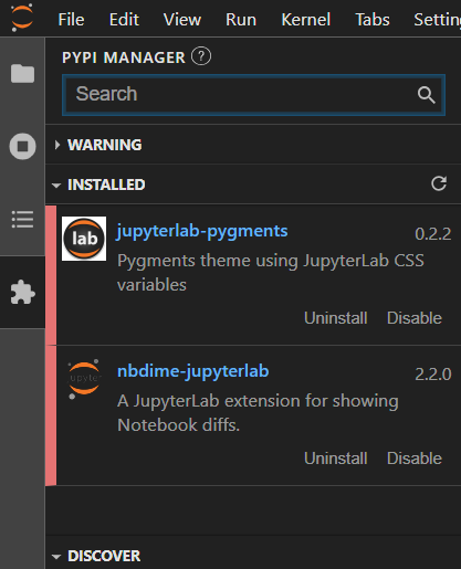
You can install extensions that increase the functionality of JupyterLab by visiting the Extensions tab.
Coming back to the example scripts from earlier, there are two ways to work with them in JupyterLab.
Using magic commands
Using the terminal
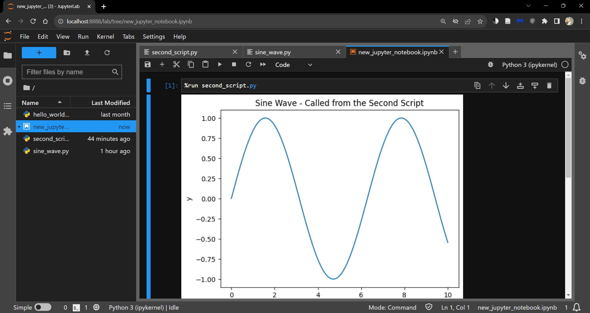
20.4.1. Using magic commands#
Jupyter Notebooks and JupyterLab support the use of magic commands - commands that extend the capabilities of a standard Jupyter Notebook.
The %run magic command allows you to run a Python script from within a Notebook.
This is a convenient way to run scripts that you are working on in the same directory as your Notebook and present the outputs within the Notebook.
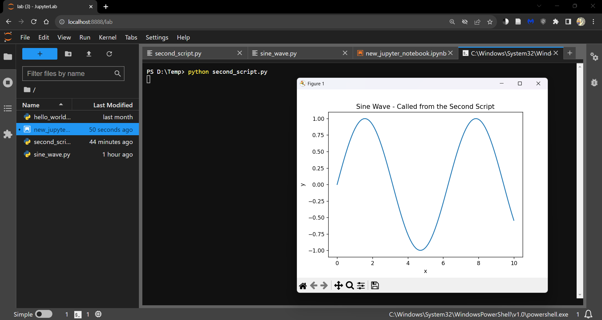
20.4.2. Using the terminal#
However, if you are looking into just running the .py file, it is sometimes easier to use the terminal.
Open a terminal from the launcher and run the following command.
> python <path to file.py>
Note
You can also run the script line by line by opening an ipykernel console either
from the launcher
by right clicking within the Notebook and selecting Create Console for Editor
Use Shift + Enter to run a line of code.
20.5. A walk through Visual Studio Code#
Visual Studio Code (VS Code) is a code editor and development workspace that can run
in the browser.
as a local installation.
Both interfaces are identical.
When you launch VS Code, you will see the following interface.
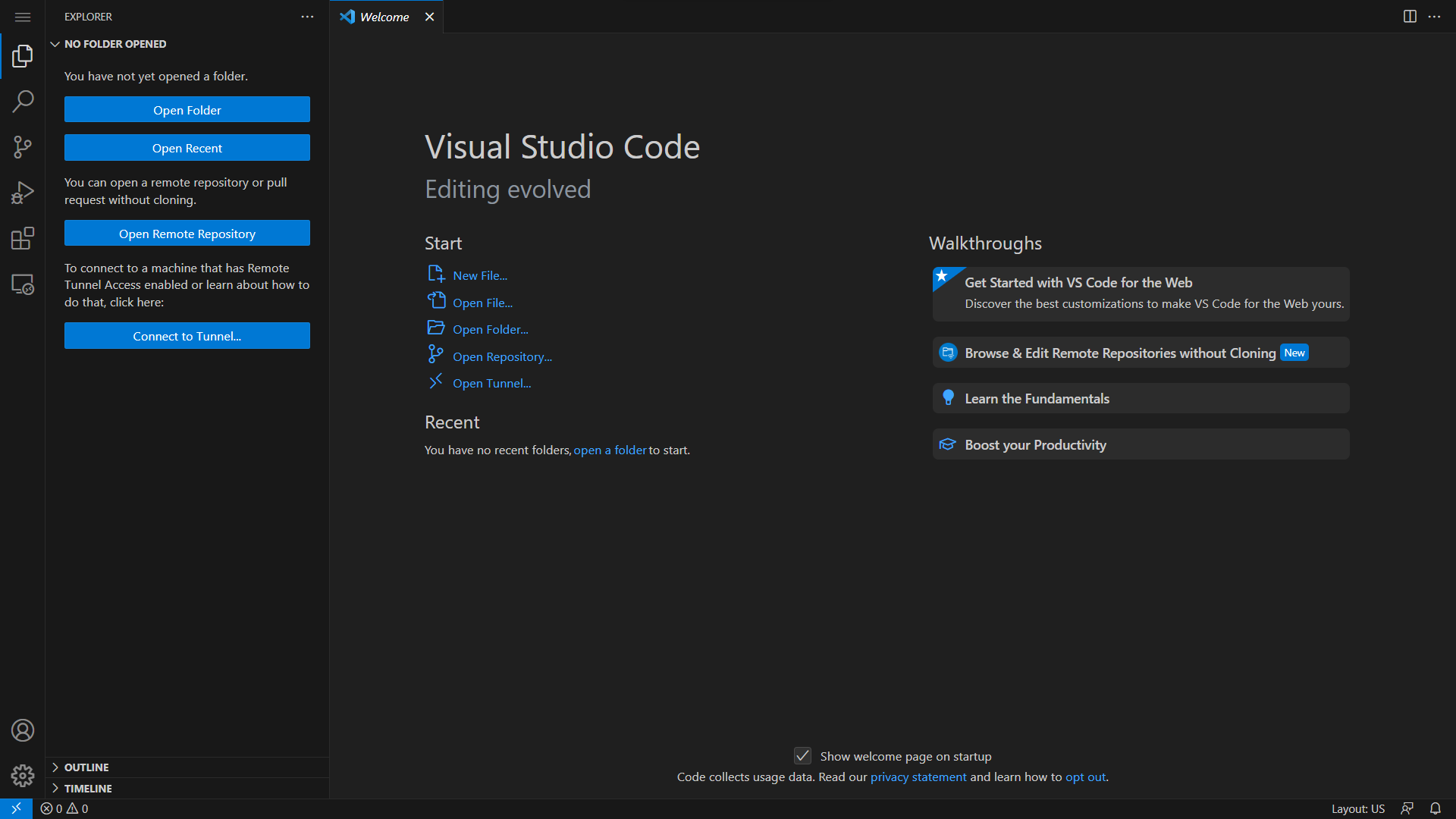
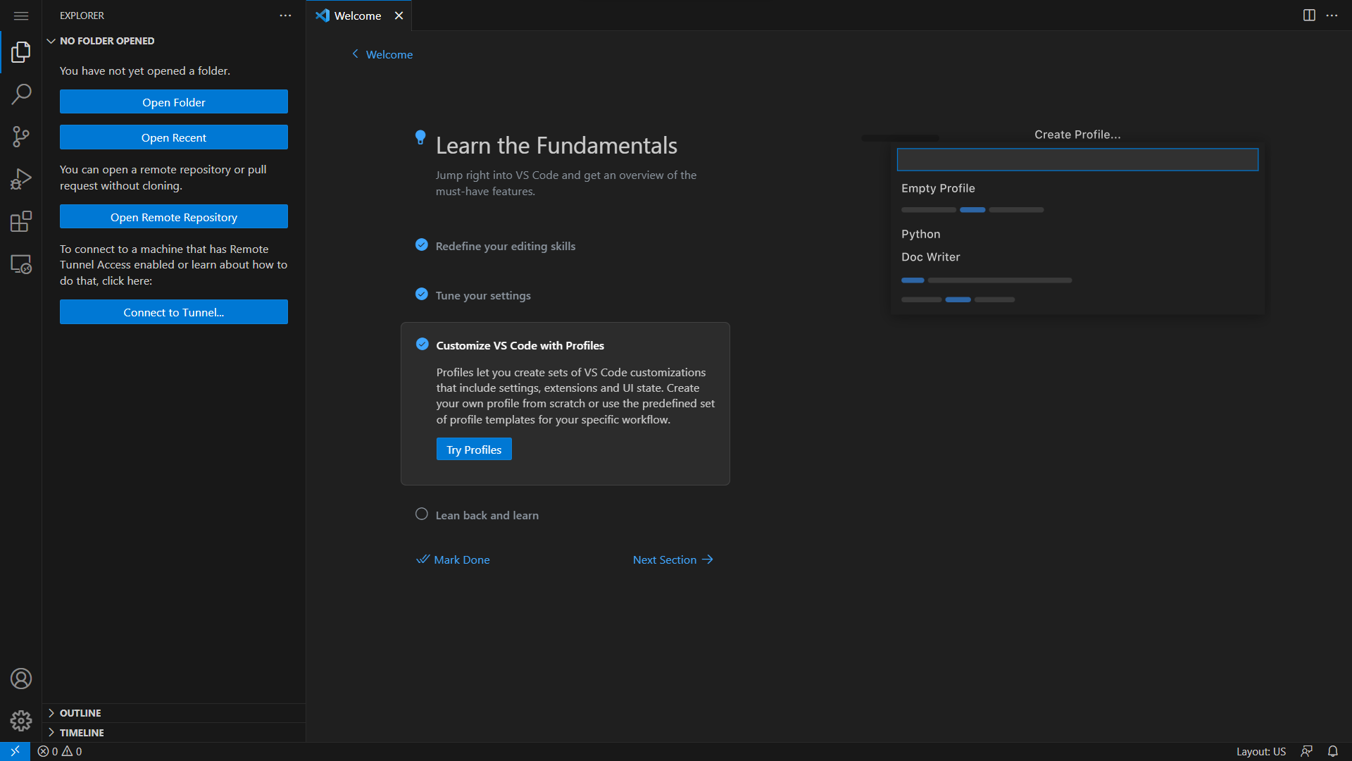
Explore how to customize VS Code to your liking through the guided walkthroughs.
When presented with the following prompt, go ahead an install all recommended extensions.
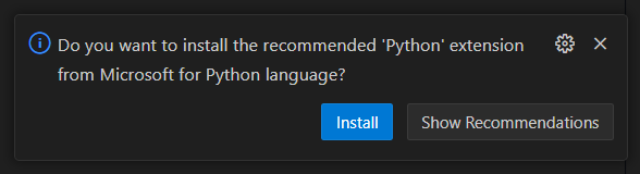
You can also install extensions from the Extensions tab.
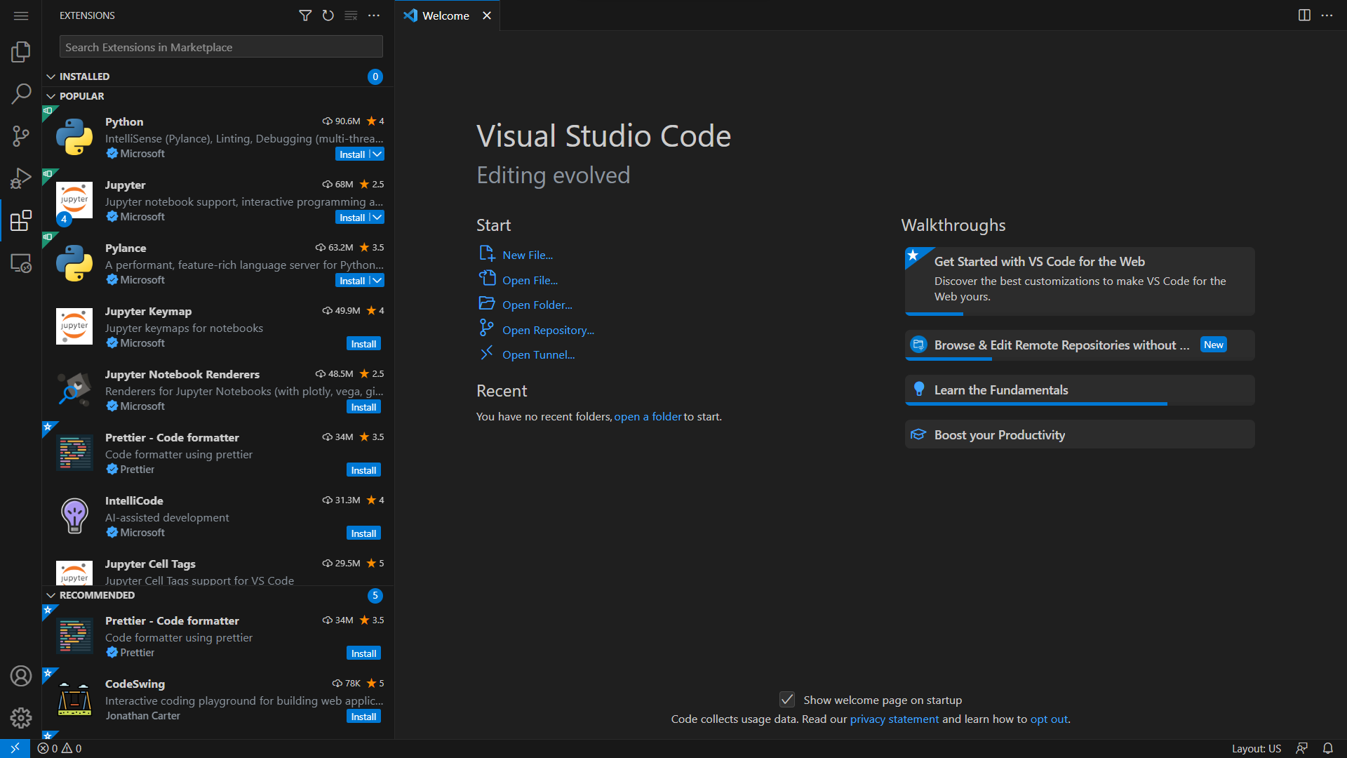
Jupyter Notebooks (.ipynb files) can be worked on in VS Code.
Make sure to install the Jupyter extension from the Extensions tab before you try to open a Jupyter Notebook.
Create a new file (in the file Explorer tab) and save it with the .ipynb extension.
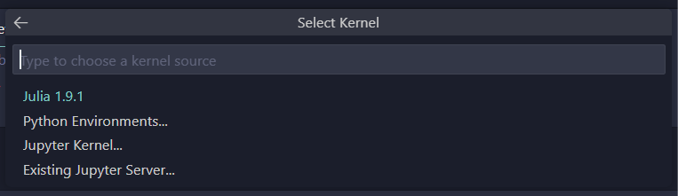
Choose a kernel/environment to run the Notebook in by clicking on the Select Kernel button on the top right corner of the editor.
VS Code also has excellent version control functionality through the Source Control tab.
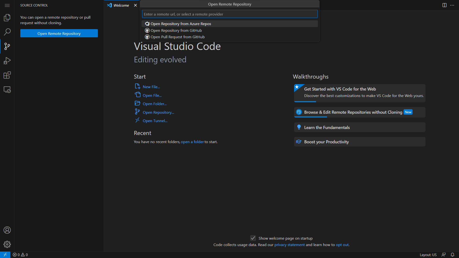
Link your GitHub account to VS Code to push and pull changes to and from your repositories.
Further discussions about version control can be found in the next section.
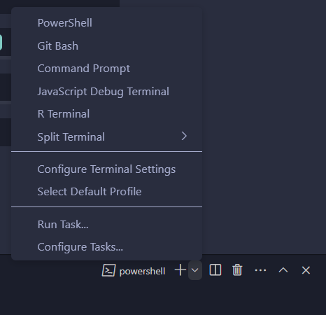
To open a new Terminal in VS Code, click on the Terminal tab and select New Terminal.
VS Code opens a new Terminal in the same directory you are working in - a PowerShell in Windows and a Bash in Linux.
You can change the shell or open a new instance through the dropdown menu on the right end of the terminal tab.
VS Code helps you manage conda environments without using the command line.
Open the Command Palette (CTRL + SHIFT + P or from the dropdown menu under View tab) and search for Python: Select Interpreter.
This loads existing environments.
You can also create new environments using Python: Create Environment in the Command Palette.
A new environment (.conda folder) is created in the the current working directory.
Coming to the example scripts from earlier, there are again two ways to work with them in VS Code.
Using the run button
Using the terminal
20.5.1. Using the run button#
You can run the script by clicking on the run button on the top right corner of the editor.
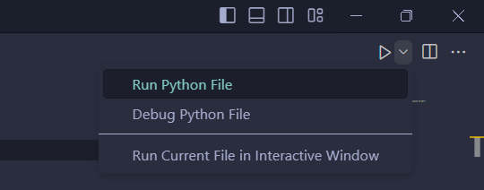
You can also run the script interactively by selecting the Run Current File in Interactive Window option from the dropdown.
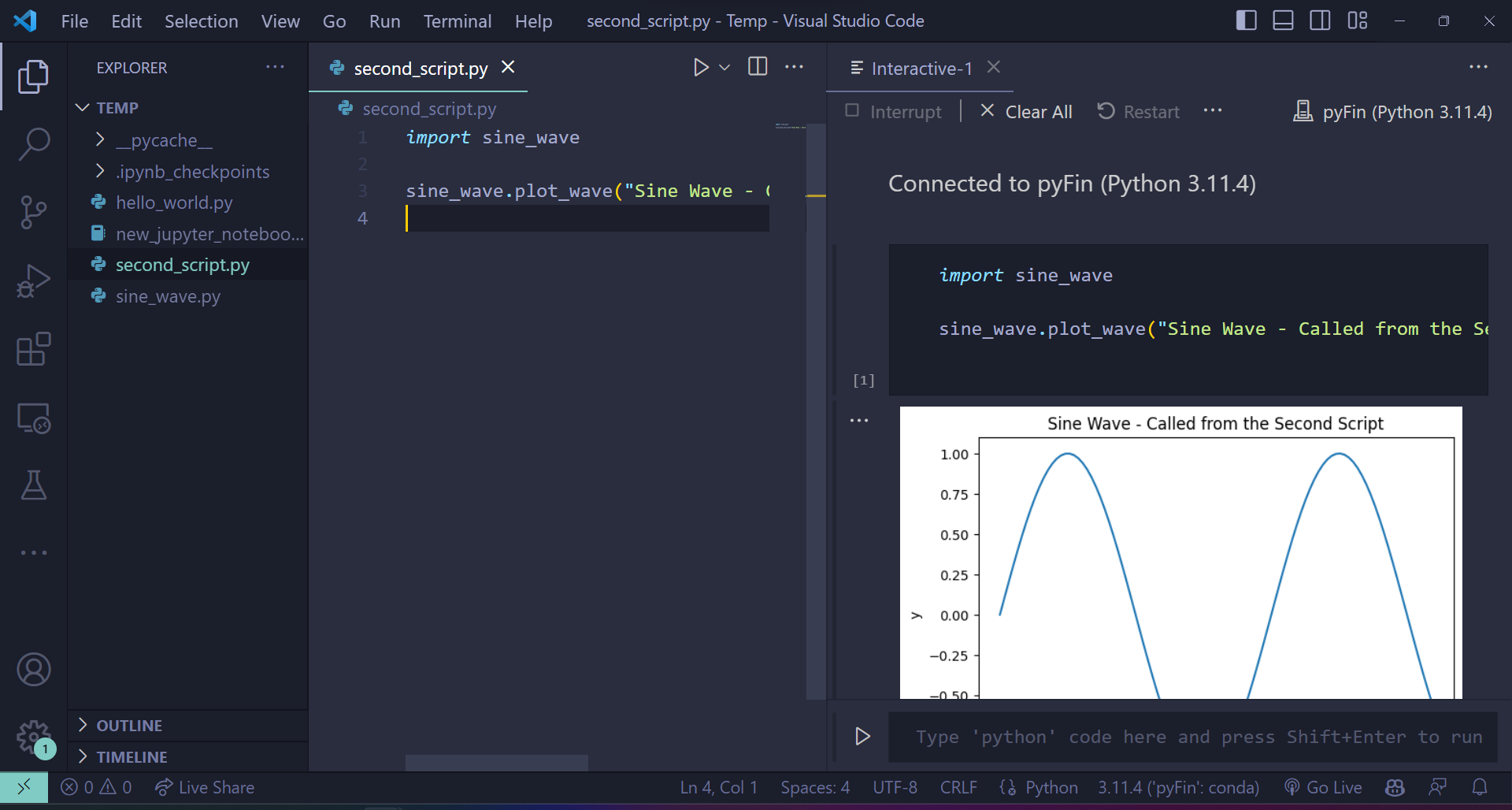
This creates an ipykernel console and runs the script.
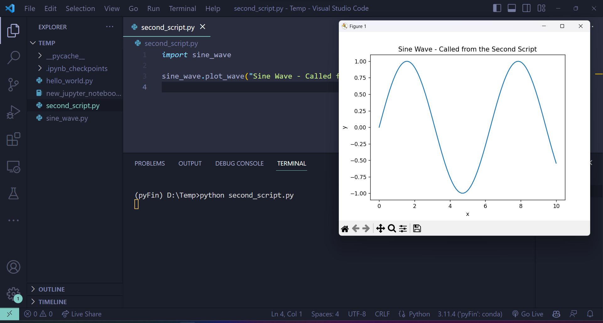
20.5.2. Using the terminal#
The command python <path to file.py> is executed on the console of your choice.
If you are using a Windows machine, you can either use the Anaconda Prompt or the Command Prompt - but, generally not the PowerShell.
Here’s an execution of the earlier code.
Note
If you would like to develop packages and build tools using Python, you may want to look into the use of Docker containers and VS Code.
However, this is outside the focus of these lectures.
20.6. Git your hands dirty#
This section will familiarize you with git and GitHub.
Git is a version control system — a piece of software used to manage digital projects such as code libraries.
In many cases, the associated collections of files — called repositories — are stored on GitHub.
GitHub is a wonderland of collaborative coding projects.
For example, it hosts many of the scientific libraries we’ll be using later on, such as this one.
Git is the underlying software used to manage these projects.
Git is an extremely powerful tool for distributed collaboration — for example, we use it to share and synchronize all the source files for these lectures.
There are two main flavors of Git
the plain vanilla command line Git version
the various point-and-click GUI versions
See, for example, the GitHub version or Git GUI integrated into your IDE.
In case you already haven’t, try
Installing Git.
Getting a copy of QuantEcon.py using Git.
For example, if you’ve installed the command line version, open up a terminal and enter.
git clone https://github.com/QuantEcon/QuantEcon.py
(This is just git clone in front of the URL for the repository)
This command will download all necessary components to rebuild the lecture you are reading now.
As the 2nd task,
Sign up to GitHub.
Look into ‘forking’ GitHub repositories (forking means making your own copy of a GitHub repository, stored on GitHub).
Fork QuantEcon.py.
Clone your fork to some local directory, make edits, commit them, and push them back up to your forked GitHub repo.
If you made a valuable improvement, send us a pull request!
For reading on these and other topics, try
Reading through the docs on GitHub.
Pro Git Book by Scott Chacon and Ben Straub.
One of the thousands of Git tutorials on the Net.