2. Getting Started #

Contents

Getting Started

2.1. Overview #

In this lecture, you will learn how to

use Python in the cloud
get a local Python environment up and running
execute simple Python commands
run a sample program
install the code libraries that underpin these lectures

2.2. Python in the Cloud #

The easiest way to get started coding in Python is by running it in the cloud.

(That is, by using a remote server that already has Python installed.)

One option that’s both free and reliable is Google Colab.

Colab also has the advantage of providing GPUs, which we will make use of in more advanced lectures.

Tutorials on how to get started with Google Colab can be found by web and video searches.

Most of our lectures include a “Launch notebook” button (with a play icon) on the top right connects you to an executable version on Colab.

2.3. Local Install #

Local installs are preferable if you have access to a suitable machine and plan to do a substantial amount of Python programming.

At the same time, local installs require more work than a cloud option like Colab.

The rest of this lecture runs you through the some details associated with local installs.

2.3.1. The Anaconda Distribution#

The core Python package is easy to install but not what you should choose for these lectures.

These lectures require the entire scientific programming ecosystem, which

the core installation doesn’t provide
is painful to install one piece at a time.

Hence the best approach for our purposes is to install a Python distribution that contains

the core Python language and
compatible versions of the most popular scientific libraries.

The best such distribution is Anaconda Python.

Anaconda is

very popular
cross-platform
comprehensive
completely unrelated to the Nicki Minaj song of the same name

Anaconda also comes with a package management system to organize your code libraries.

All of what follows assumes that you adopt this recommendation!

2.3.2. Installing Anaconda#

To install Anaconda, download the binary and follow the instructions.

Important points:

Make sure you install the correct version for your OS.
If you are asked during the installation process whether you’d like to make Anaconda your default Python installation, say yes.

2.3.3. Updating Anaconda#

Anaconda supplies a tool called conda to manage and upgrade your Anaconda packages.

One conda command you should execute regularly is the one that updates the whole Anaconda distribution.

As a practice run, please execute the following

Open up a terminal
Type conda update anaconda

For more information on conda, type conda help in a terminal.

2.4. Jupyter Notebooks #

Jupyter notebooks are one of the many possible ways to interact with Python and the scientific libraries.

They use a browser-based interface to Python with

The ability to write and execute Python commands.
Formatted output in the browser, including tables, figures, animation, etc.
The option to mix in formatted text and mathematical expressions.

Because of these features, Jupyter is now a major player in the scientific computing ecosystem.

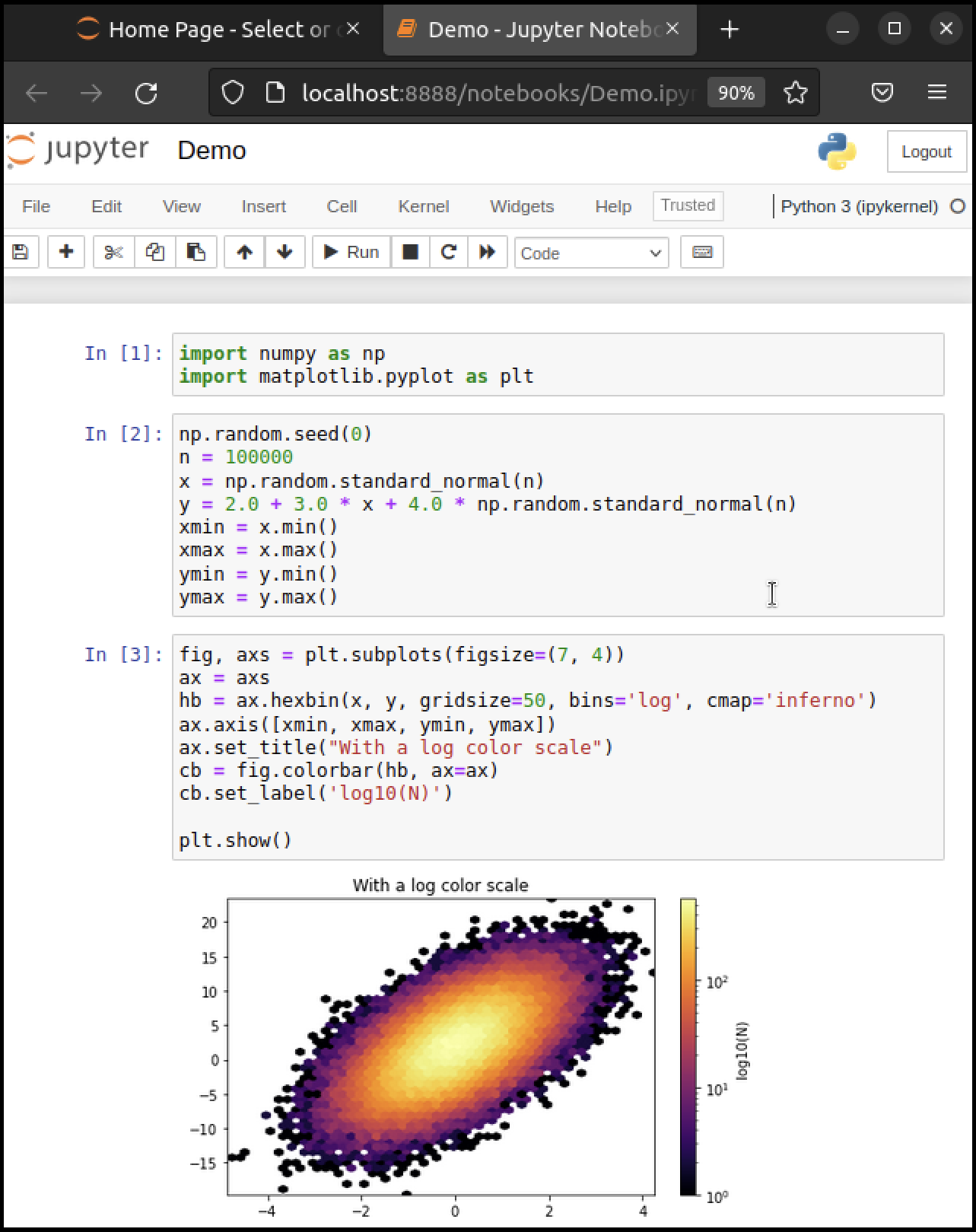
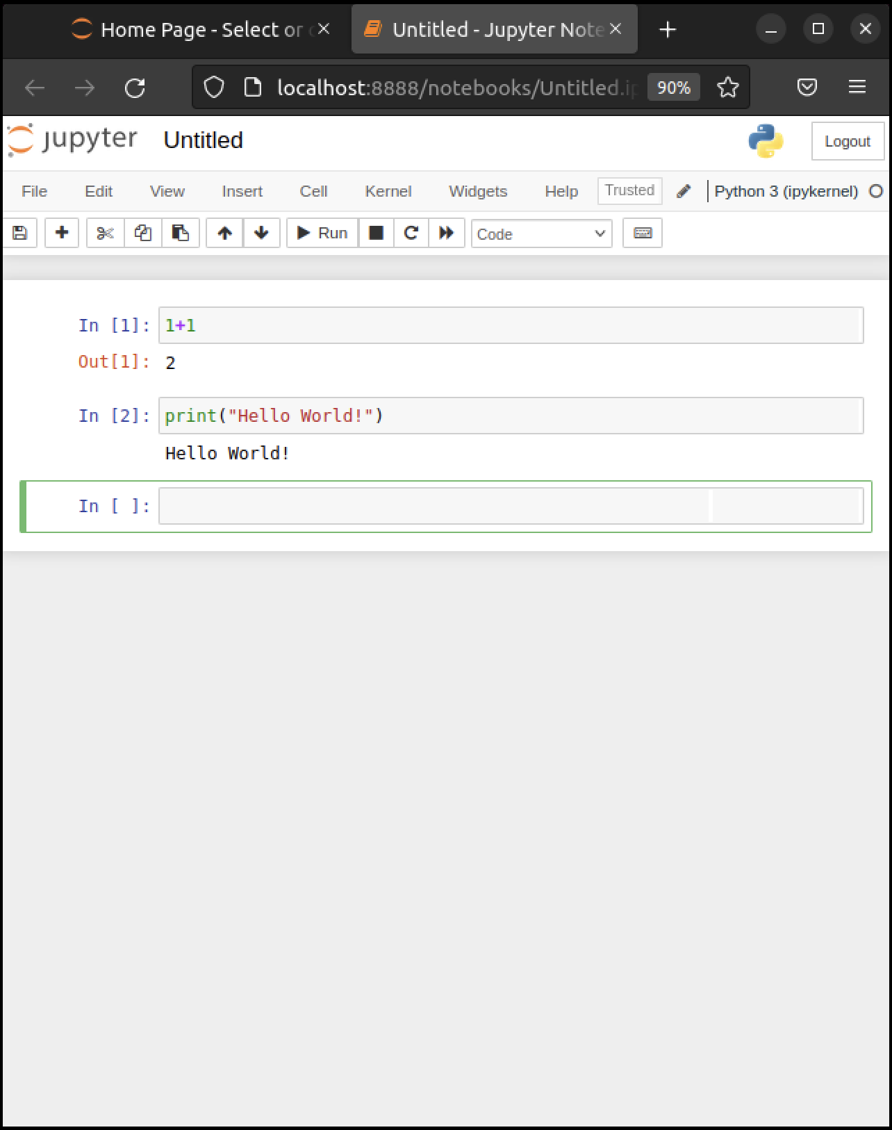
Here’s an image showing execution of some code (borrowed from here) in a Jupyter notebook

While Jupyter isn’t the only way to code in Python, it’s great for when you wish to

start coding in Python
test new ideas or interact with small pieces of code
use powerful online interactive environments such as Google Colab
share or collaborate scientific ideas with students or colleagues

These lectures are designed for executing in Jupyter notebooks.

2.4.1. Starting the Jupyter Notebook#

Once you have installed Anaconda, you can start the Jupyter notebook.

Either

search for Jupyter in your applications menu, or
open up a terminal and type jupyter notebook
- Windows users should substitute “Anaconda command prompt” for “terminal” in the previous line.

If you use the second option, you will see something like this

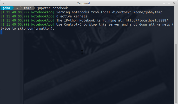
The output tells us the notebook is running at http://localhost:8888/

localhost is the name of the local machine
8888 refers to port number 8888 on your computer

Thus, the Jupyter kernel is listening for Python commands on port 8888 of our local machine.

Hopefully, your default browser has also opened up with a web page that looks something like this

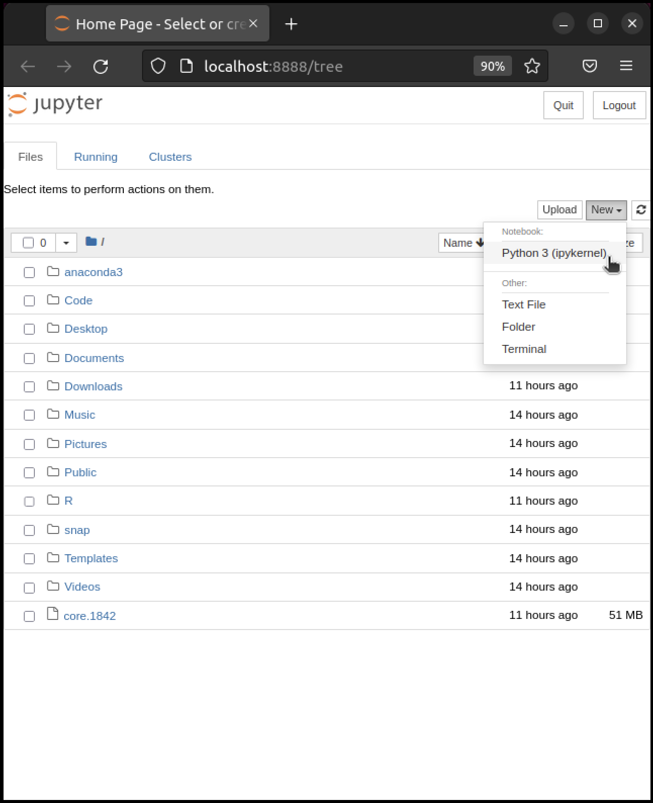
What you see here is called the Jupyter dashboard.

If you look at the URL at the top, it should be localhost:8888 or similar, matching the message above.

Assuming all this has worked OK, you can now click on New at the top right and select Python 3 or similar.

Here’s what shows up on our machine:

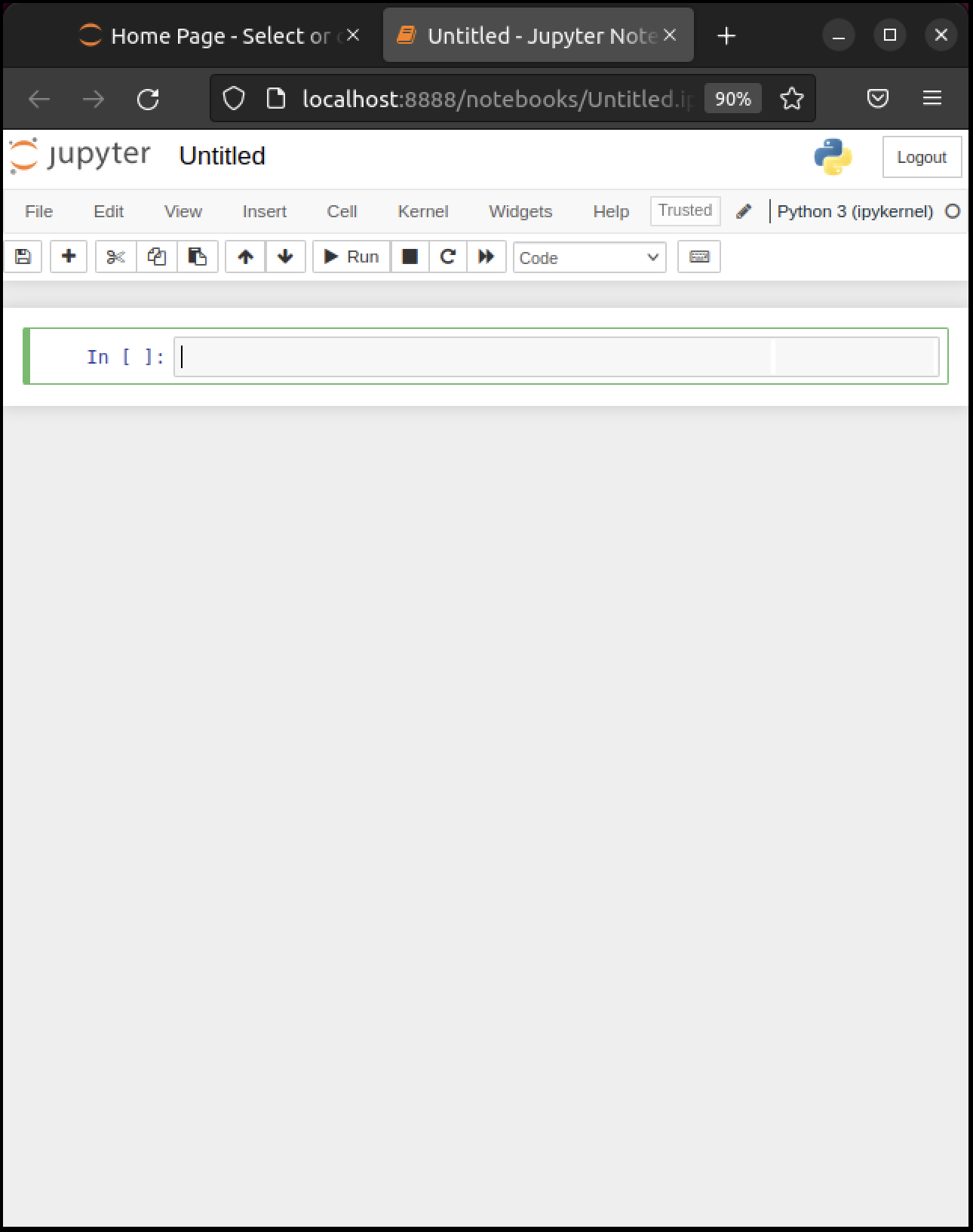
The notebook displays an active cell, into which you can type Python commands.

2.4.2. Notebook Basics#

Let’s start with how to edit code and run simple programs.

2.4.2.1. Running Cells#

Notice that, in the previous figure, the cell is surrounded by a green border.

This means that the cell is in edit mode.

In this mode, whatever you type will appear in the cell with the flashing cursor.

When you’re ready to execute the code in a cell, hit Shift-Enter instead of the usual Enter.

Note

There are also menu and button options for running code in a cell that you can find by exploring.

2.4.2.3. Inserting Unicode (e.g., Greek Letters)#

Python supports unicode, allowing the use of characters such as \(\alpha\) and \(\beta\) as names in your code.

In a code cell, try typing \alpha and then hitting the tab key on your keyboard.

2.4.2.4. A Test Program#

Let’s run a test program.

Here’s an arbitrary program we can use: http://matplotlib.org/3.1.1/gallery/pie_and_polar_charts/polar_bar.html.

On that page, you’ll see the following code

import numpy as np
import matplotlib.pyplot as plt
%matplotlib inline
plt.rcParams['figure.figsize'] = (10,6)

# Fixing random state for reproducibility
np.random.seed(19680801)

# Compute pie slices
N = 20
θ = np.linspace(0.0, 2 * np.pi, N, endpoint=False)
radii = 10 * np.random.rand(N)
width = np.pi / 4 * np.random.rand(N)
colors = plt.cm.viridis(radii / 10.)

ax = plt.subplot(111, projection='polar')
ax.bar(θ, radii, width=width, bottom=0.0, color=colors, alpha=0.5)

plt.show()

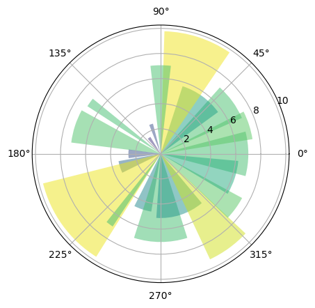
_images/655c5f8a564fafbb579f408637a2fb55a8559fefad9e066598f00dd0c1e81582.png

Don’t worry about the details for now — let’s just run it and see what happens.

The easiest way to run this code is to copy and paste it into a cell in the notebook.

Hopefully you will get a similar plot.

2.4.3. Working with the Notebook#

Here are a few more tips on working with Jupyter notebooks.

2.4.3.1. Tab Completion#

In the previous program, we executed the line import numpy as np

NumPy is a numerical library we’ll work with in depth.

After this import command, functions in NumPy can be accessed with np.function_name type syntax.

For example, try np.random.randn(3).

We can explore these attributes of np using the Tab key.

For example, here we type np.random.r and hit Tab

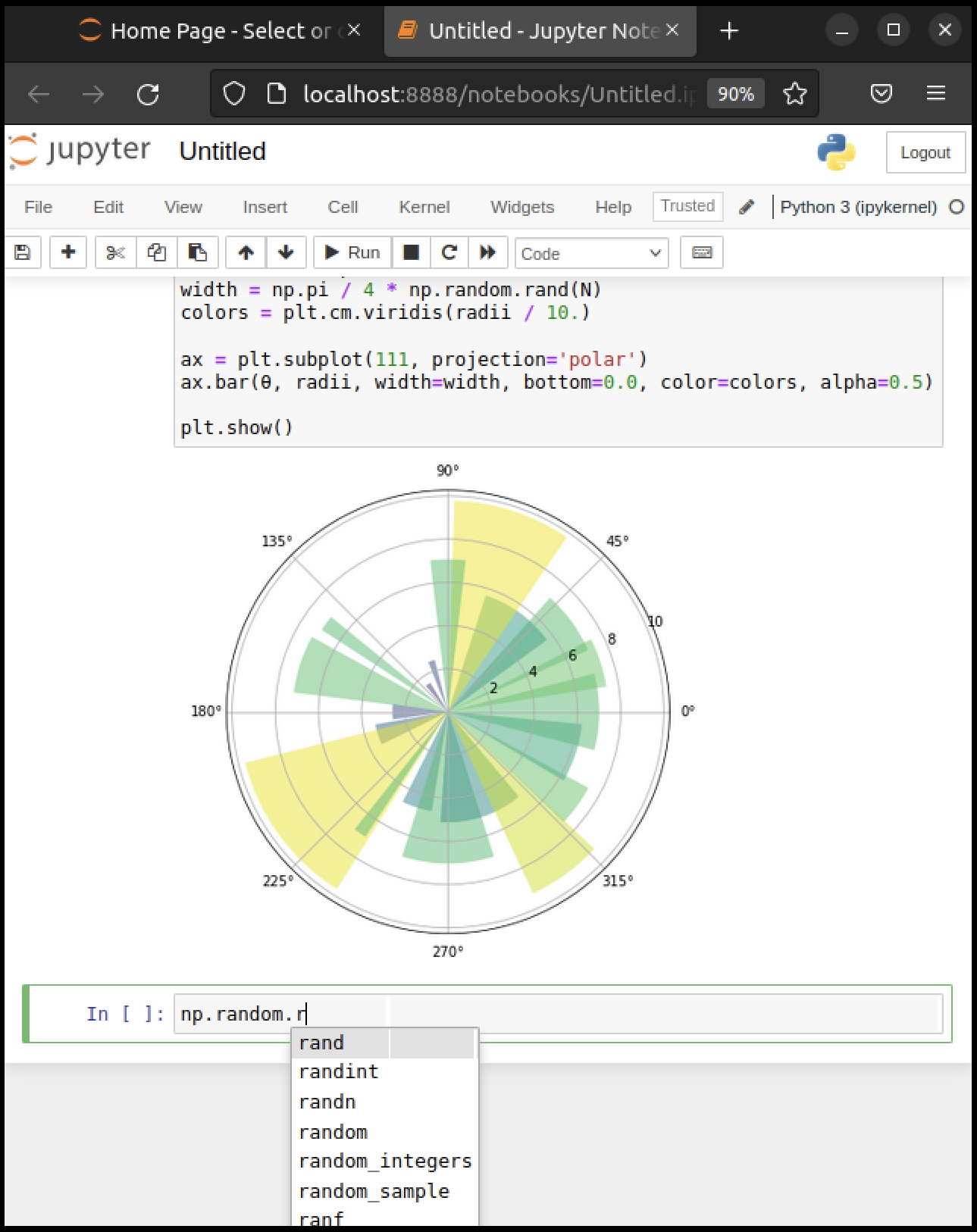
Jupyter offers several possible completions for you to choose from.

In this way, the Tab key helps remind you of what’s available and also saves you typing.

2.4.3.2. On-Line Help#

To get help on np.random.randn, we can execute np.random.randn?.

Documentation appears in a split window of the browser, like so

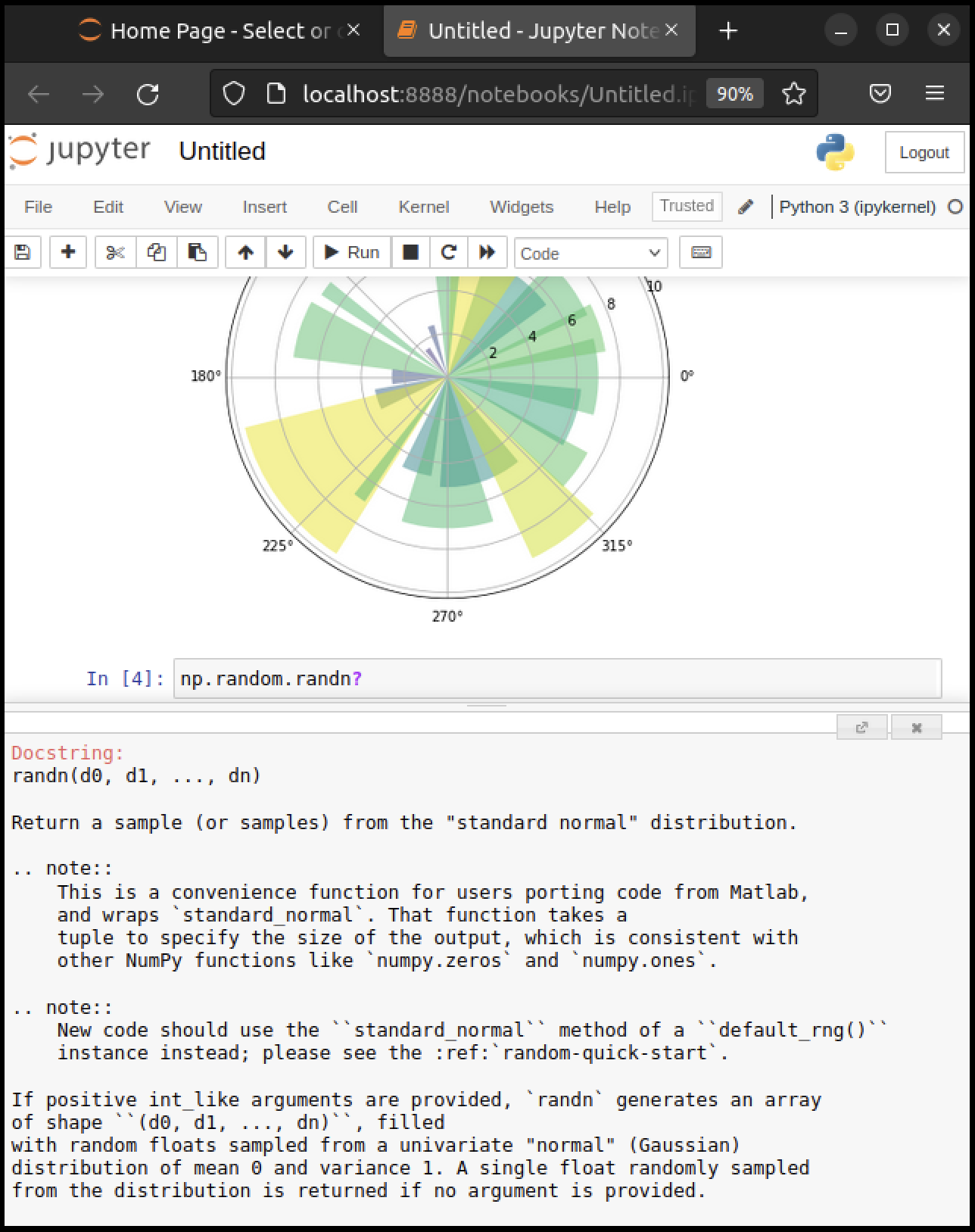
Clicking on the top right of the lower split closes the on-line help.

We will learn more about how to create documentation like this later!

2.4.3.3. Other Content#

In addition to executing code, the Jupyter notebook allows you to embed text, equations, figures and even videos in the page.

For example, we can enter a mixture of plain text and LaTeX instead of code.

Next we Esc to enter command mode and then type m to indicate that we are writing Markdown, a mark-up language similar to (but simpler than) LaTeX.

(You can also use your mouse to select Markdown from the Code drop-down box just below the list of menu items)

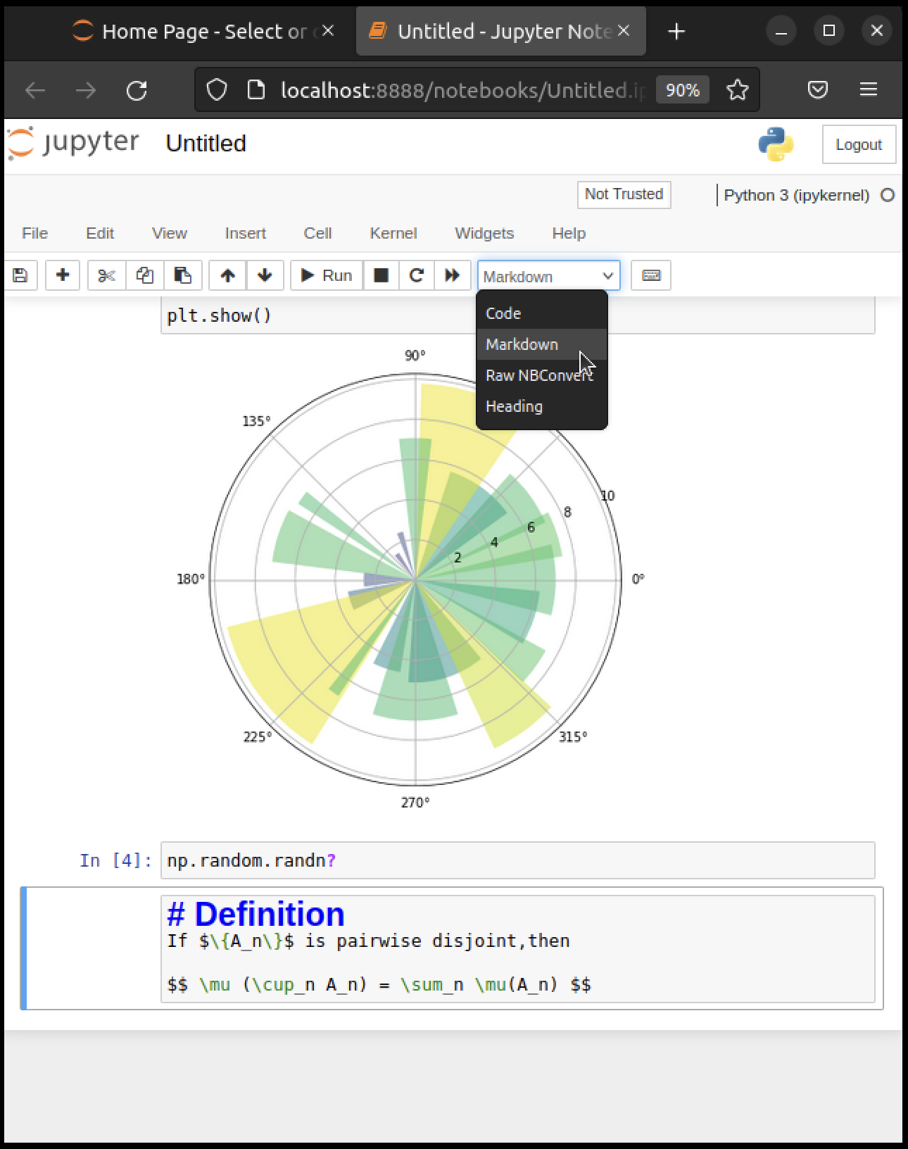
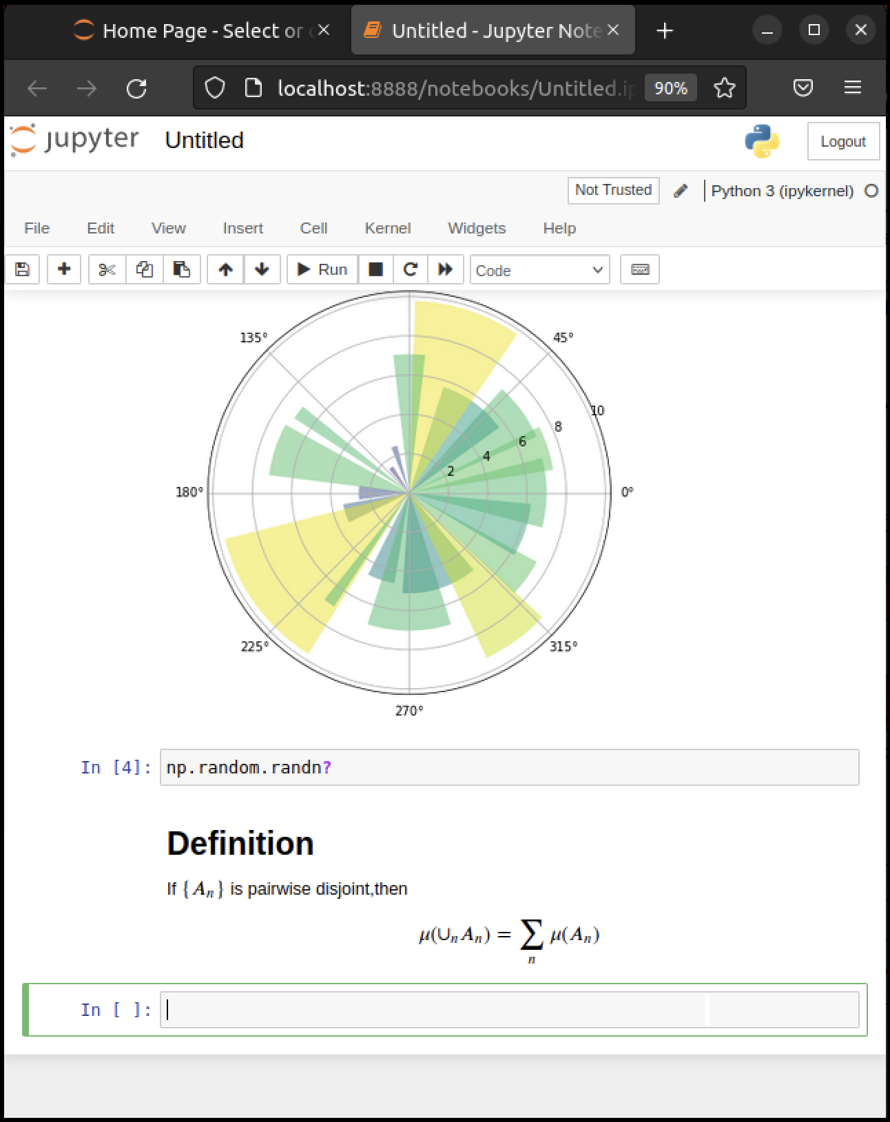
Now we Shift+Enter to produce this

2.4.4. Debugging Code#

Debugging is the process of identifying and removing errors from a program.

You will spend a lot of time debugging code, so it is important to learn how to do it effectively.

If you are using a newer version of Jupyter, you should see a bug icon on the right end of the toolbar.

Clicking this icon will enable the Jupyter debugger.

Note

You may also need to open the Debugger Panel (View -> Debugger Panel).

You can set breakpoints by clicking on the line number of the cell you want to debug.

When you run the cell, the debugger will stop at the breakpoint.

You can then step through the code line by line using the buttons on the “Next” button on the CALLSTACK toolbar (located in the right hand window).

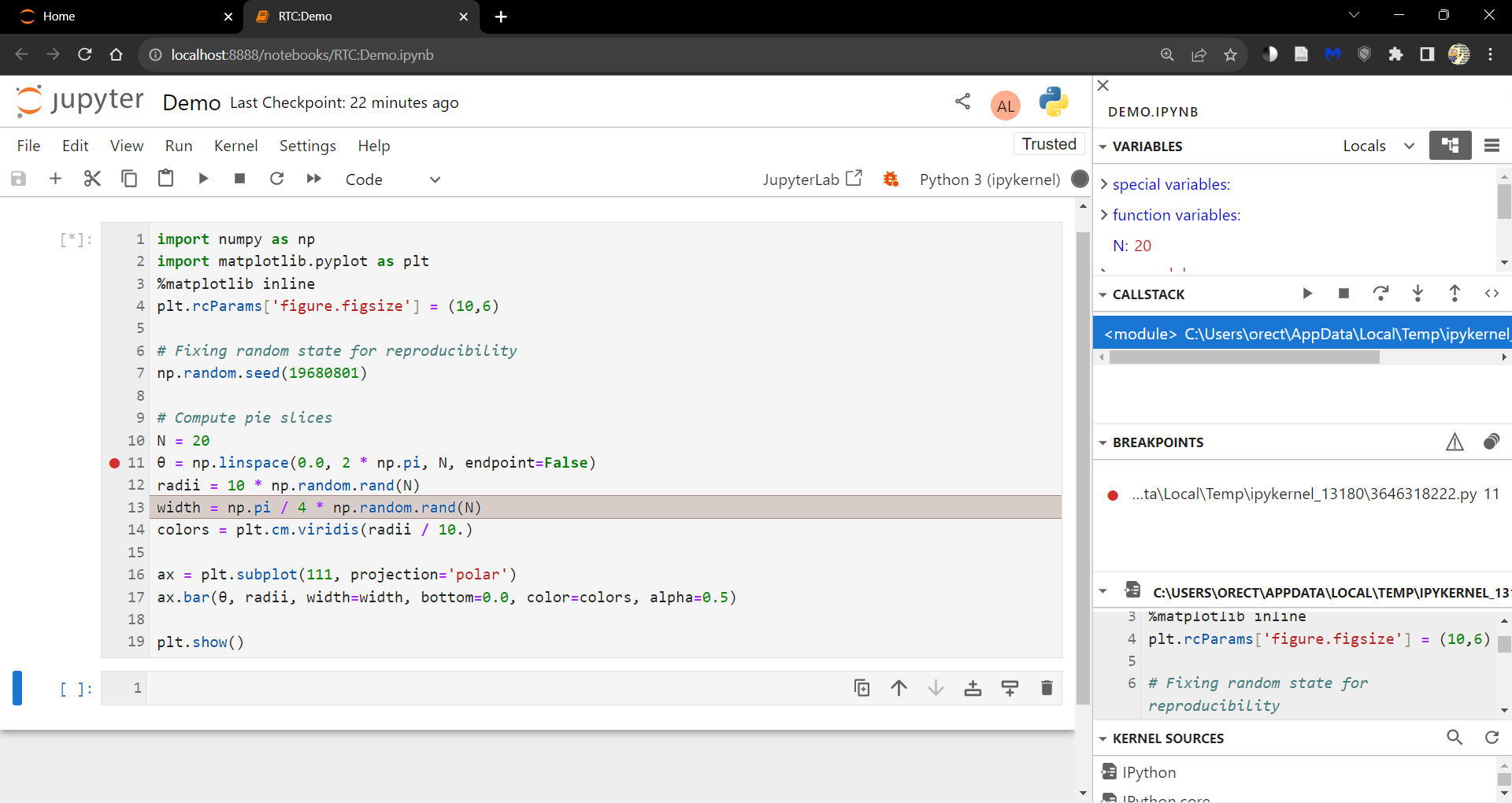
You can explore more functionality of the debugger in the Jupyter documentation.

2.4.6. QuantEcon Notes#

QuantEcon has its own site for sharing Jupyter notebooks related to economics – QuantEcon Notes.

Notebooks submitted to QuantEcon Notes can be shared with a link, and are open to comments and votes by the community.

2.5. Installing Libraries #

Most of the libraries we need come in Anaconda.

Other libraries can be installed with pip or conda.

One library we’ll be using is QuantEcon.py.

You can install QuantEcon.py by starting Jupyter and typing

!conda install quantecon

into a cell.

Alternatively, you can type the following into a terminal

conda install quantecon

More instructions can be found on the library page.

To upgrade to the latest version, which you should do regularly, use

conda upgrade quantecon

Another library we will be using is interpolation.py.

This can be installed by typing in Jupyter

!conda install -c conda-forge interpolation

2.6. Working with Python Files #

So far we’ve focused on executing Python code entered into a Jupyter notebook cell.

Traditionally most Python code has been run in a different way.

Code is first saved in a text file on a local machine

By convention, these text files have a .py extension.

We can create an example of such a file as follows:

%%writefile foo.py

print("foobar")

Writing foo.py

This writes the line print("foobar") into a file called foo.py in the local directory.

Here %%writefile is an example of a cell magic.

2.6.1. Editing and Execution#

If you come across code saved in a *.py file, you’ll need to consider the following questions:

how should you execute it?
How should you modify or edit it?

2.6.1.1. Option 1: JupyterLab#

JupyterLab is an integrated development environment built on top of Jupyter notebooks.

With JupyterLab you can edit and run *.py files as well as Jupyter notebooks.

To start JupyterLab, search for it in the applications menu or type jupyter-lab in a terminal.

Now you should be able to open, edit and run the file foo.py created above by opening it in JupyterLab.

Read the docs or search for a recent YouTube video to find more information.

2.6.1.2. Option 2: Using a Text Editor#

One can also edit files using a text editor and then run them from within Jupyter notebooks.

A text editor is an application that is specifically designed to work with text files — such as Python programs.

Nothing beats the power and efficiency of a good text editor for working with program text.

A good text editor will provide

efficient text editing commands (e.g., copy, paste, search and replace)
syntax highlighting, etc.

Right now, an extremely popular text editor for coding is VS Code.

VS Code is easy to use out of the box and has many high quality extensions.

Alternatively, if you want an outstanding free text editor and don’t mind a seemingly vertical learning curve plus long days of pain and suffering while all your neural pathways are rewired, try Vim.

2.7. Exercises #

Exercise 2.1

If Jupyter is still running, quit by using Ctrl-C at the terminal where you started it.

Now launch again, but this time using jupyter notebook --no-browser.

This should start the kernel without launching the browser.

Note also the startup message: It should give you a URL such as http://localhost:8888 where the notebook is running.

Now

Start your browser — or open a new tab if it’s already running.
Enter the URL from above (e.g. http://localhost:8888) in the address bar at the top.

You should now be able to run a standard Jupyter notebook session.

This is an alternative way to start the notebook that can also be handy.

This can also work when you accidentally close the webpage as long as the kernel is still running.

2.3.1. The Anaconda Distribution#

2.3.2. Installing Anaconda#

2.3.3. Updating Anaconda#

2.4.1. Starting the Jupyter Notebook#

2.4.2. Notebook Basics#

2.4.2.1. Running Cells#

2.4.2.2. Modal Editing#

2.4.2.3. Inserting Unicode (e.g., Greek Letters)#

2.4.2.4. A Test Program#

2.4.3. Working with the Notebook#

2.4.3.1. Tab Completion#

2.4.3.2. On-Line Help#

2.4.3.3. Other Content#

2.4.4. Debugging Code#

2.4.5. Sharing Notebooks#

2.4.6. QuantEcon Notes#

2.6.1. Editing and Execution#

2.6.1.1. Option 1: JupyterLab#

2.6.1.2. Option 2: Using a Text Editor#