13. Numba#

In addition to what’s in Anaconda, this lecture will need the following libraries:

!pip install quantecon

Please also make sure that you have the latest version of Anaconda, since old versions are a common source of errors.

Let’s start with some imports:

import numpy as np
import quantecon as qe
import matplotlib.pyplot as plt

13.1. Overview#

In an earlier lecture we discussed vectorization, which can improve execution speed by sending array processing operations in batch to efficient low-level code.

However, as discussed in that lecture, traditional vectorization schemes have weaknesses:

Highly memory-intensive for compound array operations
Ineffective or impossible for some algorithms

One way to circumvent these problems is by using Numba, a just in time (JIT) compiler for Python.

Numba compiles functions to native machine code instructions at runtime.

When it succeeds, the result is performance comparable to compiled C or Fortran.

In addition, Numba can do useful tricks such as multithreading.

This lecture introduces the core ideas.

Note

Some readers might be curious about the relationship between Numba and Julia, which contains its own JIT compiler. While the two compilers are similar in many ways, Numba is less ambitious, attempting only to compile a small subset of the Python language. Although this might sound like a deficiency, it is also a strength: the more restrictive nature of Numba makes it easy to use well and good at what it does.

13.2. Compiling Functions#

13.2.1. An Example#

Let’s consider a problem that’s difficult to vectorize (i.e., hand off to array processing operations).

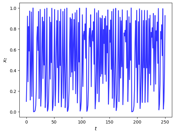
The problem involves generating the trajectory via the quadratic map

\[ x_{t+1} = \alpha x_t (1 - x_t) \]

In what follows we set \(\alpha = 4\).

13.2.1.1. Base Version#

Here’s the plot of a typical trajectory, starting from \(x_0 = 0.1\), with \(t\) on the x-axis

def qm(x0, n, α=4.0):
    x = np.empty(n+1)
    x[0] = x0
    for t in range(n):
      x[t+1] = α * x[t] * (1 - x[t])
    return x

x = qm(0.1, 250)
fig, ax = plt.subplots()
ax.plot(x, 'b-', lw=2, alpha=0.8)
ax.set_xlabel('$t$', fontsize=12)
ax.set_ylabel('$x_{t}$', fontsize = 12)
plt.show()

_images/7ee1041b5cfbccf2c054e0d597571f59456d08103b80b433cd2523aa05b6a94a.png

Let’s see how long this takes to run for large \(n\)

n = 10_000_000

with qe.Timer() as timer1:
    # Time Python base version
    x = qm(0.1, n)

4.7526 seconds elapsed

13.2.1.2. Acceleration via Numba#

To speed the function qm up using Numba, we first import the jit function

from numba import jit

Now we apply it to qm, producing a new function:

qm_numba = jit(qm)

The function qm_numba is a version of qm that is “targeted” for JIT-compilation.

We will explain what this means momentarily.

Let’s time this new version:

with qe.Timer() as timer2:
    # Time jitted version
    x = qm_numba(0.1, n)

0.2150 seconds elapsed

This is a large speed gain.

In fact, the next time and all subsequent times it runs even faster as the function has been compiled and is in memory:

with qe.Timer() as timer3:
    # Second run
    x = qm_numba(0.1, n)

0.0723 seconds elapsed

Here’s the speed gain

timer1.elapsed /  timer3.elapsed

65.73277274900661

This is a big boost for a small modification to our original code.

Let’s discuss how this works.

13.2.2. How and When it Works#

Numba attempts to generate fast machine code using the infrastructure provided by the LLVM Project.

It does this by inferring type information on the fly.

(See our earlier lecture on scientific computing for a discussion of types.)

The basic idea is this:

Python is very flexible and hence we could call the function qm with many types.
- e.g., x0 could be a NumPy array or a list, n could be an integer or a float, etc.
This makes it very difficult to generate efficient machine code ahead of time (i.e., before runtime).
However, when we do actually call the function, say by running qm(0.5, 10), the types of x0, α and n are determined.
Moreover, the types of other variables in qm can be inferred once the input types are known.
So the strategy of Numba and other JIT compilers is to wait until the function is called, and then compile.

That is called “just-in-time” compilation.

Note that, if you make the call qm_numba(0.5, 10) and then follow it with qm_numba(0.9, 20), compilation only takes place on the first call.

This is because compiled code is cached and reused as required.

This is why, in the code above, the second run of qm_numba is faster.

Remark

In practice, rather than writing qm_numba = jit(qm), we typically use decorator syntax and put @jit before the function definition. This is equivalent to adding qm = jit(qm) after the definition.

13.3. Sharp Bits#

Numba is relatively easy to use but not always seamless.

Let’s review some of the issues users run into.

13.3.1. Typing#

Successful type inference is the key to JIT compilation.

In an ideal setting, Numba can infer all necessary type information.

When Numba cannot infer all type information, it will raise an error.

For example, in the setting below, Numba is unable to determine the type of the function g when compiling iterate

@jit
def iterate(f, x0, n):
    x = x0
    for t in range(n):
        x = f(x)
    return x

# Not jitted
def g(x):
    return np.cos(x) - 2 * np.sin(x)

# This code throws an error
try:
    iterate(g, 0.5, 100)
except Exception as e:
    print(e)

Failed in nopython mode pipeline (step: nopython frontend)
non-precise type pyobject
During: typing of argument at /tmp/ipykernel_2605/946716698.py (1)

File "../../../../../../tmp/ipykernel_2605/946716698.py", line 1:
<source missing, REPL/exec in use?>

During: Pass nopython_type_inference 

This error may have been caused by the following argument(s):
- argument 0: Cannot determine Numba type of <class 'function'>

In the present case, we can fix this easily by compiling g.

@jit
def g(x):
    return np.cos(x) - 2 * np.sin(x)

iterate(g, 0.5, 100)

2.223875299559663

In other cases, such as when we want to use functions from external libaries such as SciPy, there might not be any easy workaround.

13.3.2. Global Variables#

Another thing to be careful about when using Numba is handling of global variables.

For example, consider the following code

a = 1

@jit
def add_a(x):
    return a + x

print(add_a(10))

a = 2

print(add_a(10))

Notice that changing the global had no effect on the value returned by the function 😱.

When Numba compiles machine code for functions, it treats global variables as constants to ensure type stability.

To avoid this, pass values as function arguments rather than relying on globals.

13.4. Multithreaded Loops in Numba#

In addition to JIT compilation, Numba provides support for parallel computing on CPUs and GPUs.

The key tool for parallelization on CPUs in Numba is the prange function, which tells Numba to execute loop iterations in parallel across available cores.

To illustrate, let’s look first at a simple, single-threaded (i.e., non-parallelized) piece of code.

The code simulates updating the wealth \(w_t\) of a household via the rule

\[ w_{t+1} = R_{t+1} s w_t + y_{t+1} \]

Here

\(R\) is the gross rate of return on assets
\(s\) is the savings rate of the household and
\(y\) is labor income.

We model both \(R\) and \(y\) as independent draws from a lognormal distribution.

Here’s the code:

@jit
def update(w, r=0.1, s=0.3, v1=0.1, v2=1.0):
    " Updates household wealth. "
    # Draw shocks
    R = np.exp(v1 * np.random.randn()) * (1 + r)
    y = np.exp(v2 * np.random.randn())
    # Update wealth
    w = R * s * w + y
    return w

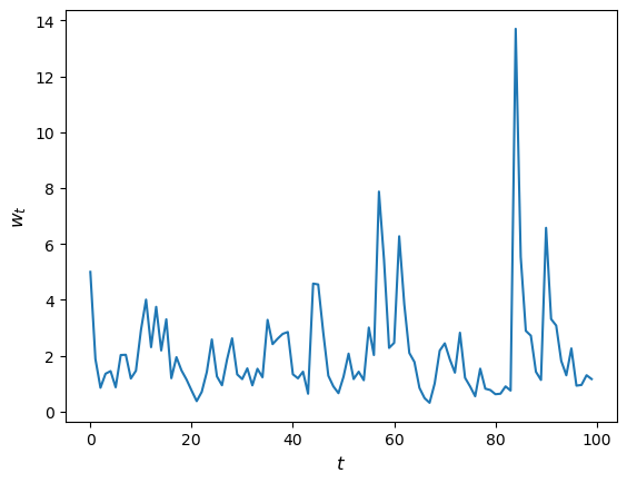
Let’s have a look at how wealth evolves under this rule.

fig, ax = plt.subplots()

T = 100
w = np.empty(T)
w[0] = 5
for t in range(T-1):
    w[t+1] = update(w[t])

ax.plot(w)
ax.set_xlabel('$t$', fontsize=12)
ax.set_ylabel('$w_{t}$', fontsize=12)
plt.show()

_images/097a471e9836ed0314944e38700700b9cf2232c7d0862c82d179cd76d2dc6806.png

Now let’s suppose that we have a large population of households and we want to know what median wealth will be.

This is not easy to solve with pencil and paper, so we will use simulation instead:

Simulate a large number of households forward in time
Calculate median wealth

Here’s the code:

@jit
def compute_long_run_median(w0=1, T=1000, num_reps=50_000):
    obs = np.empty(num_reps)
    # For each household
    for i in range(num_reps):
        # Set the initial condition and run forward in time
        w = w0
        for t in range(T):
            w = update(w)
        # Record the final value
        obs[i] = w
    # Take the median of all final values
    return np.median(obs)

Let’s see how fast this runs:

with qe.Timer():
    # Warm up
    compute_long_run_median()

6.7708 seconds elapsed

with qe.Timer():
    # Second run
    compute_long_run_median()

5.6576 seconds elapsed

To speed this up, we’re going to parallelize it via multithreading.

To do so, we add the parallel=True flag and change range to prange:

from numba import prange

@jit(parallel=True)
def compute_long_run_median_parallel(
        w0=1, T=1000, num_reps=50_000
    ):
    obs = np.empty(num_reps)
    for i in prange(num_reps):  # Parallelize over households
        w = w0
        for t in range(T):
            w = update(w)
        obs[i] = w
    return np.median(obs)

Let’s look at the timing:

with qe.Timer():
    # Warm up
    compute_long_run_median_parallel()

1.1379 seconds elapsed

with qe.Timer():
    # Second run
    compute_long_run_median_parallel()

0.5847 seconds elapsed

The speed-up is significant.

Notice that we parallelize across households rather than over time – updates of an individual household across time periods are inherently sequential.

For GPU-based parallelization, see our lectures on JAX.

13.5. Exercises#

Exercise 13.1

Previously we considered how to approximate \(\pi\) by Monte Carlo.

Use the same idea here, but make the code efficient using Numba.

Compare speed with and without Numba when the sample size is large.

Solution

Here is one solution:

@jit
def calculate_pi(n=1_000_000):
    count = 0
    for i in range(n):
        u, v = np.random.uniform(0, 1), np.random.uniform(0, 1)
        d = np.sqrt((u - 0.5)**2 + (v - 0.5)**2)
        if d < 0.5:
            count += 1

    area_estimate = count / n
    return area_estimate * 4  # dividing by radius**2

Now let’s see how fast it runs:

with qe.Timer():
    calculate_pi()

0.1888 seconds elapsed

with qe.Timer():
    calculate_pi()

0.0325 seconds elapsed

If we switch off JIT compilation by removing @jit, the code takes around 150 times as long on our machine.

So we get a speed gain of 2 orders of magnitude by adding four characters.

Exercise 13.2

In the Introduction to Quantitative Economics with Python lecture series you can learn all about finite-state Markov chains.

For now, let’s just concentrate on simulating a very simple example of such a chain.

Suppose that the volatility of returns on an asset can be in one of two regimes — high or low.

The transition probabilities across states are as follows

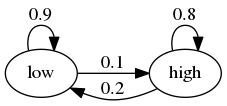
For example, let the period length be one day, and suppose the current state is high.

We see from the graph that the state tomorrow will be

high with probability 0.8
low with probability 0.2

Your task is to simulate a sequence of daily volatility states according to this rule.

Set the length of the sequence to n = 1_000_000 and start in the high state.

Implement a pure Python version and a Numba version, and compare speeds.

To test your code, evaluate the fraction of time that the chain spends in the low state.

If your code is correct, it should be about 2/3.

Hint

Represent the low state as 0 and the high state as 1.
If you want to store integers in a NumPy array and then apply JIT compilation, use x = np.empty(n, dtype=np.int64).

Solution

We let

0 represent “low”
1 represent “high”

p, q = 0.1, 0.2  # Prob of leaving low and high state respectively

Here’s a pure Python version of the function

def compute_series(n):
    x = np.empty(n, dtype=np.int64)
    x[0] = 1  # Start in state 1
    U = np.random.uniform(0, 1, size=n)
    for t in range(1, n):
        current_x = x[t-1]
        if current_x == 0:
            x[t] = U[t] < p
        else:
            x[t] = U[t] > q
    return x

Let’s run this code and check that the fraction of time spent in the low state is about 0.666

n = 1_000_000
x = compute_series(n)
print(np.mean(x == 0))  # Fraction of time x is in state 0

0.668164

This is (approximately) the right output.

Now let’s time it:

with qe.Timer():
    compute_series(n)

0.6043 seconds elapsed

Next let’s implement a Numba version, which is easy

compute_series_numba = jit(compute_series)

Let’s check we still get the right numbers

x = compute_series_numba(n)
print(np.mean(x == 0))

0.665486

Let’s see the time

with qe.Timer():
    compute_series_numba(n)

0.0215 seconds elapsed

This is a nice speed improvement for one line of code!

Exercise 13.3

In an earlier exercise, we used Numba to accelerate an effort to compute the constant \(\pi\) by Monte Carlo.

Now try adding parallelization and see if you get further speed gains.

You should not expect huge gains here because, while there are many independent tasks (draw point and test if in circle), each one has low execution time.

Generally speaking, parallelization is less effective when the individual tasks to be parallelized are very small relative to total execution time.

This is due to overheads associated with spreading all of these small tasks across multiple CPUs.

Nevertheless, with suitable hardware, it is possible to get nontrivial speed gains in this exercise.

For the size of the Monte Carlo simulation, use something substantial, such as n = 100_000_000.

Solution

Here is one solution:

@jit(parallel=True)
def calculate_pi(n=1_000_000):
    count = 0
    for i in prange(n):
        u, v = np.random.uniform(0, 1), np.random.uniform(0, 1)
        d = np.sqrt((u - 0.5)**2 + (v - 0.5)**2)
        if d < 0.5:
            count += 1

    area_estimate = count / n
    return area_estimate * 4  # dividing by radius**2

Now let’s see how fast it runs:

with qe.Timer():
    calculate_pi()

0.4759 seconds elapsed

with qe.Timer():
    calculate_pi()

0.0046 seconds elapsed

By switching parallelization on and off (selecting True or False in the @jit annotation), we can test the speed gain that multithreading provides on top of JIT compilation.

On our workstation, we find that parallelization increases execution speed by a factor of 2 or 3.

(If you are executing locally, you will get different numbers, depending mainly on the number of CPUs on your machine.)

Exercise 13.4

In our lecture on SciPy, we discussed pricing a call option in a setting where the underlying stock price had a simple and well-known distribution.

Here we discuss a more realistic setting.

We recall that the price of the option obeys

\[ P = \beta^n \mathbb E \max\{ S_n - K, 0 \} \]

where

\(\beta\) is a discount factor,
\(n\) is the expiry date,
\(K\) is the strike price and
\(\{S_t\}\) is the price of the underlying asset at each time \(t\).

Suppose that n, β, K = 20, 0.99, 100.

Assume that the stock price obeys

\[ \ln \frac{S_{t+1}}{S_t} = \mu + \sigma_t \xi_{t+1} \]

where

\[ \sigma_t = \exp(h_t), \quad h_{t+1} = \rho h_t + \nu \eta_{t+1} \]

Here \(\{\xi_t\}\) and \(\{\eta_t\}\) are IID and standard normal.

(This is a stochastic volatility model, where the volatility \(\sigma_t\) varies over time.)

Use the defaults μ, ρ, ν, S0, h0 = 0.0001, 0.1, 0.001, 10, 0.

(Here S0 is \(S_0\) and h0 is \(h_0\).)

By generating \(M\) paths \(s_0, \ldots, s_n\), compute the Monte Carlo estimate

\[ \hat P_M := \beta^n \mathbb E \max\{ S_n - K, 0 \} \approx \frac{1}{M} \sum_{m=1}^M \max \{S_n^m - K, 0 \} \]

of the price, applying Numba and parallelization.

Solution

With \(s_t := \ln S_t\), the price dynamics become

\[ s_{t+1} = s_t + \mu + \exp(h_t) \xi_{t+1} \]

Using this fact, the solution can be written as follows.

M = 10_000_000

n, β, K = 20, 0.99, 100
μ, ρ, ν, S0, h0 = 0.0001, 0.1, 0.001, 10, 0

@jit(parallel=True)
def compute_call_price_parallel(β=β,
                                μ=μ,
                                S0=S0,
                                h0=h0,
                                K=K,
                                n=n,
                                ρ=ρ,
                                ν=ν,
                                M=M):
    current_sum = 0.0
    # For each sample path
    for m in prange(M):
        s = np.log(S0)
        h = h0
        # Simulate forward in time
        for t in range(n):
            s = s + μ + np.exp(h) * np.random.randn()
            h = ρ * h + ν * np.random.randn()
        # And add the value max{S_n - K, 0} to current_sum
        current_sum += max(np.exp(s) - K, 0)

    return β**n * current_sum / M

Try swapping between parallel=True and parallel=False and noting the run time.

If you are on a machine with many CPUs, the difference should be significant.