15. SymPy #

Contents

SymPy

15.1. Overview #

Unlike numerical libraries that deal with values, SymPy focuses on manipulating mathematical symbols and expressions directly.

SymPy provides a wide range of features including

symbolic expression
equation solving
simplification
calculus
matrices
discrete math, etc.

These functions make SymPy a popular open-source alternative to other proprietary symbolic computational software such as Mathematica.

In this lecture, we will explore some of the functionality of SymPy and demonstrate how to use basic SymPy functions to solve economic models.

15.2. Getting Started #

Let’s first import the library and initialize the printer for symbolic output

from sympy import *
from sympy.plotting import plot, plot3d_parametric_line, plot3d
from sympy.solvers.inequalities import reduce_rational_inequalities
from sympy.stats import Poisson, Exponential, Binomial, density, moment, E, cdf

import numpy as np
import matplotlib.pyplot as plt

# Enable the mathjax printer
init_printing(use_latex='mathjax')

15.3. Symbolic algebra #

15.3.1. Symbols#

First we initialize some symbols to work with

x, y, z = symbols('x y z')

Symbols are the basic units for symbolic computation in SymPy.

15.3.2. Expressions#

We can now use symbols x, y, and z to build expressions and equations.

Here we build a simple expression first

expr = (x+y) ** 2
expr

\[\displaystyle \left(x + y\right)^{2}\]

We can expand this expression with the expand function

expand_expr = expand(expr)
expand_expr

\[\displaystyle x^{2} + 2 x y + y^{2}\]

and factorize it back to the factored form with the factor function

factor(expand_expr)

\[\displaystyle \left(x + y\right)^{2}\]

We can solve this expression

solve(expr)

\[\displaystyle \left[ \left\{ x : - y\right\}\right]\]

Note this is equivalent to solving the following equation for x

\[ (x + y)^2 = 0 \]

Note

Solvers is an important module with tools to solve different types of equations.

There are a variety of solvers available in SymPy depending on the nature of the problem.

15.3.3. Equations#

SymPy provides several functions to manipulate equations.

Let’s develop an equation with the expression we defined before

eq = Eq(expr, 0)
eq

\[\displaystyle \left(x + y\right)^{2} = 0\]

Solving this equation with respect to \(x\) gives the same output as solving the expression directly

solve(eq, x)

\[\displaystyle \left[ - y\right]\]

SymPy can handle equations with multiple solutions

eq = Eq(expr, 1)
solve(eq, x)

\[\displaystyle \left[ 1 - y, \ - y - 1\right]\]

solve function can also combine multiple equations together and solve a system of equations

eq2 = Eq(x, y)
eq2

\[\displaystyle x = y\]

solve([eq, eq2], [x, y])

\[\displaystyle \left[ \left( - \frac{1}{2}, \ - \frac{1}{2}\right), \ \left( \frac{1}{2}, \ \frac{1}{2}\right)\right]\]

We can also solve for the value of \(y\) by simply substituting \(x\) with \(y\)

expr_sub = expr.subs(x, y)
expr_sub

\[\displaystyle 4 y^{2}\]

solve(Eq(expr_sub, 1))

\[\displaystyle \left[ - \frac{1}{2}, \ \frac{1}{2}\right]\]

Below is another example equation with the symbol x and functions sin, cos, and tan using the Eq function

# Create an equation
eq = Eq(cos(x) / (tan(x)/sin(x)), 0)
eq

\[\displaystyle \frac{\sin{\left(x \right)} \cos{\left(x \right)}}{\tan{\left(x \right)}} = 0\]

Now we simplify this equation using the simplify function

# Simplify an expression
simplified_expr = simplify(eq)
simplified_expr

\[\displaystyle \cos^{2}{\left(x \right)} = 0\]

Again, we use the solve function to solve this equation

# Solve the equation
sol = solve(eq, x)
sol

\[\displaystyle \left[ \frac{\pi}{2}, \ \frac{3 \pi}{2}\right]\]

SymPy can also handle more complex equations involving trigonometry and complex numbers.

We demonstrate this using Euler’s formula

# 'I' represents the imaginary number i 
euler = cos(x) + I*sin(x)
euler

\[\displaystyle i \sin{\left(x \right)} + \cos{\left(x \right)}\]

simplify(euler)

\[\displaystyle e^{i x}\]

If you are interested, we encourage you to read the lecture on trigonometry and complex numbers.

15.3.3.1. Example: fixed point computation#

Fixed point computation is frequently used in economics and finance.

Here we solve the fixed point of the Solow-Swan growth dynamics:

\[ k_{t+1}=s f\left(k_t\right)+(1-\delta) k_t, \quad t=0,1, \ldots \]

where \(k_t\) is the capital stock, \(f\) is a production function, \(\delta\) is a rate of depreciation.

We are interested in calculating the fixed point of this dynamics, i.e., the value of \(k\) such that \(k_{t+1} = k_t\).

With \(f(k) = Ak^\alpha\), we can show the unique fixed point of the dynamics \(k^*\) using pen and paper:

\[ k^*:=\left(\frac{s A}{\delta}\right)^{1 /(1-\alpha)} \]

This can be easily computed in SymPy

A, s, k, α, δ = symbols('A s k^* α δ')

Now we solve for the fixed point \(k^*\)

\[ k^* = sA(k^*)^{\alpha}+(1-\delta) k^* \]

# Define Solow-Swan growth dynamics
solow = Eq(s*A*k**α + (1-δ)*k, k)
solow

\[\displaystyle A \left(k^{*}\right)^{α} s + k^{*} \left(1 - δ\right) = k^{*}\]

solve(solow, k)

\[\displaystyle \left[ \left(\frac{A s}{δ}\right)^{- \frac{1}{α - 1}}\right]\]

15.3.4. Inequalities and logic#

SymPy also allows users to define inequalities and set operators and provides a wide range of operations.

reduce_inequalities([2*x + 5*y <= 30, 4*x + 2*y <= 20], [x])

\[\displaystyle x \leq 5 - \frac{y}{2} \wedge x \leq 15 - \frac{5 y}{2} \wedge -\infty < x\]

And(2*x + 5*y <= 30, x > 0)

\[\displaystyle 2 x + 5 y \leq 30 \wedge x > 0\]

15.3.5. Series#

Series are widely used in economics and statistics, from asset pricing to the expectation of discrete random variables.

We can construct a simple series of summations using Sum function and Indexed symbols

x, y, i, j = symbols("x y i j")
sum_xy = Sum(Indexed('x', i)*Indexed('y', j), 
            (i, 0, 3),
            (j, 0, 3))
sum_xy

\[\begin{split}\displaystyle \sum_{\substack{0 \leq i \leq 3\\0 \leq j \leq 3}} {x}_{i} {y}_{j}\end{split}\]

To evaluate the sum, we can lambdify the formula.

The lambdified expression can take numeric values as input for \(x\) and \(y\) and compute the result

sum_xy = lambdify([x, y], sum_xy)
grid = np.arange(0, 4, 1)
sum_xy(grid, grid)

15.3.5.1. Example: bank deposits#

Imagine a bank with \(D_0\) as the deposit at time \(t\).

It loans \((1-r)\) of its deposits and keeps a fraction \(r\) as cash reserves.

Its deposits over an infinite time horizon can be written as

\[ \sum_{i=0}^\infty (1-r)^i D_0 \]

Let’s compute the deposits at time \(t\)

D = symbols('D_0')
r = Symbol('r', positive=True)
Dt = Sum('(1 - r)^i * D_0', (i, 0, oo))
Dt

\[\displaystyle \sum_{i=0}^{\infty} D_{0} \left(1 - r\right)^{i}\]

We can call the doit method to evaluate the series

Dt.doit()

\[\begin{split}\displaystyle D_{0} \left(\begin{cases} \frac{1}{r} & \text{for}\: \left|{r - 1}\right| < 1 \\\sum_{i=0}^{\infty} \left(1 - r\right)^{i} & \text{otherwise} \end{cases}\right)\end{split}\]

Simplifying the expression above gives

simplify(Dt.doit())

\[\begin{split}\displaystyle \begin{cases} \frac{D_{0}}{r} & \text{for}\: r > 0 \wedge r < 2 \\D_{0} \sum_{i=0}^{\infty} \left(1 - r\right)^{i} & \text{otherwise} \end{cases}\end{split}\]

This is consistent with the solution in the lecture on geometric series.

15.3.5.2. Example: discrete random variable#

In the following example, we compute the expectation of a discrete random variable.

Let’s define a discrete random variable \(X\) following a Poisson distribution:

\[ f(x) = \frac{\lambda^x e^{-\lambda}}{x!}, \quad x = 0, 1, 2, \ldots \]

λ = symbols('lambda')

# We refine the symbol x to positive integers
x = Symbol('x', integer=True, positive=True)
pmf = λ**x * exp(-λ) / factorial(x)
pmf

\[\displaystyle \frac{\lambda^{x} e^{- \lambda}}{x!}\]

We can verify if the sum of probabilities for all possible values equals \(1\):

\[ \sum_{x=0}^{\infty} f(x) = 1 \]

sum_pmf = Sum(pmf, (x, 0, oo))
sum_pmf.doit()

\[\displaystyle 1\]

The expectation of the distribution is:

\[ E(X) = \sum_{x=0}^{\infty} x f(x) \]

fx = Sum(x*pmf, (x, 0, oo))
fx.doit()

\[\displaystyle \lambda\]

SymPy includes a statistics submodule called Stats.

Stats offers built-in distributions and functions on probability distributions.

The computation above can also be condensed into one line using the expectation function E in the Stats module

λ = Symbol("λ", positive = True)

# Using sympy.stats.Poisson() method
X = Poisson("x", λ)
E(X)

\[\displaystyle λ\]

15.4. Symbolic Calculus #

SymPy allows us to perform various calculus operations, such as limits, differentiation, and integration.

15.4.1. Limits#

We can compute limits for a given expression using the limit function

# Define an expression
f = x**2 / (x-1)

# Compute the limit
lim = limit(f, x, 0)
lim

\[\displaystyle 0\]

15.4.2. Derivatives#

We can differentiate any SymPy expression using the diff function

# Differentiate a function with respect to x
df = diff(f, x)
df

\[\displaystyle - \frac{x^{2}}{\left(x - 1\right)^{2}} + \frac{2 x}{x - 1}\]

15.4.3. Integrals#

We can compute definite and indefinite integrals using the integrate function

# Calculate the indefinite integral
indef_int = integrate(df, x)
indef_int

\[\displaystyle x + \frac{1}{x - 1}\]

Let’s use this function to compute the moment-generating function of exponential distribution with the probability density function:

\[ f(x) = \lambda e^{-\lambda x}, \quad x \ge 0 \]

λ = Symbol('lambda', positive=True)
x = Symbol('x', positive=True)
pdf = λ * exp(-λ*x)
pdf

\[\displaystyle \lambda e^{- \lambda x}\]

t = Symbol('t', positive=True)
moment_t = integrate(exp(t*x) * pdf, (x, 0, oo))
simplify(moment_t)

\[\begin{split}\displaystyle \begin{cases} \frac{\lambda}{\lambda - t} & \text{for}\: \lambda > t \wedge \frac{\lambda}{t} \neq 1 \\\lambda \int\limits_{0}^{\infty} e^{x \left(- \lambda + t\right)}\, dx & \text{otherwise} \end{cases}\end{split}\]

Note that we can also use Stats module to compute the moment

X = Exponential(x, λ)

moment(X, 1)

\[\displaystyle \frac{1}{\lambda}\]

E(X**t)

\[\displaystyle \lambda^{- t} \Gamma\left(t + 1\right)\]

Using the integrate function, we can derive the cumulative density function of the exponential distribution with \(\lambda = 0.5\)

λ_pdf = pdf.subs(λ, 1/2)
λ_pdf

\[\displaystyle 0.5 e^{- 0.5 x}\]

integrate(λ_pdf, (x, 0, 4))

\[\displaystyle 0.864664716763387\]

Using cdf in Stats module gives the same solution

cdf(X, 1/2)

\[\begin{split}\displaystyle \left( z \mapsto \begin{cases} 1 - e^{- z \lambda} & \text{for}\: z \geq 0 \\0 & \text{otherwise} \end{cases} \right)\end{split}\]

# Plug in a value for z 
λ_cdf = cdf(X, 1/2)(4)
λ_cdf

\[\displaystyle 1 - e^{- 4 \lambda}\]

# Substitute λ
λ_cdf.subs({λ: 1/2})

\[\displaystyle 0.864664716763387\]

15.5. Plotting #

SymPy provides a powerful plotting feature.

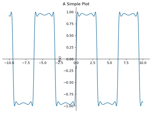
First we plot a simple function using the plot function

f = sin(2 * sin(2 * sin(2 * sin(x))))
p = plot(f, (x, -10, 10), show=False)
p.title = 'A Simple Plot'
p.show()

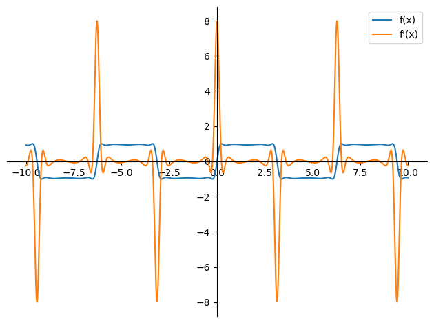
_images/74ac4762bd9e06493dbdf5020a7f61f6b7dbb416a26f59fb8c0d86623d3456ee.png

Similar to Matplotlib, SymPy provides an interface to customize the graph

plot_f = plot(f, (x, -10, 10), 
              xlabel='', ylabel='', 
              legend = True, show = False)
plot_f[0].label = 'f(x)'
df = diff(f)
plot_df = plot(df, (x, -10, 10), 
            legend = True, show = False)
plot_df[0].label = 'f\'(x)'
plot_f.append(plot_df[0])
plot_f.show()

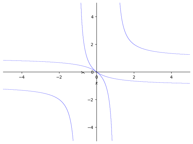
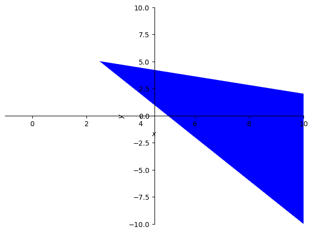
_images/610cca2e7a4830d9fda270a0fe74bf8d73c446ce93a82d0768fd842ca57c1425.png

It also supports plotting implicit functions and visualizing inequalities

p = plot_implicit(Eq((1/x + 1/y)**2, 1))

_images/fd8d9ee9d75efcff3604dc7b21ba8c4bebac7fb434eaaa8393982547f3a113ec.png

p = plot_implicit(And(2*x + 5*y <= 30, 4*x + 2*y >= 20),
                     (x, -1, 10), (y, -10, 10))

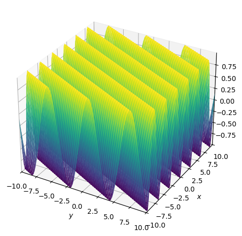
_images/47efbb2017e6d5923d2ffb078be2fa3c14812448104a1db69bee40635b1e66b7.png

and visualizations in three-dimensional space

p = plot3d(cos(2*x + y), zlabel='')

_images/f9cf50d8d921eacda60ec72f6c7e7a0791ff864c0a6f1f8e19fe151e14dbced6.png

15.6. Application: Two-person Exchange Economy #

Imagine a pure exchange economy with two people (\(a\) and \(b\)) and two goods recorded as proportions (\(x\) and \(y\)).

They can trade goods with each other according to their preferences.

Assume that the utility functions of the consumers are given by

\[ u_a(x, y) = x^{\alpha} y^{1-\alpha} \]

\[ u_b(x, y) = (1 - x)^{\beta} (1 - y)^{1-\beta} \]

where \(\alpha, \beta \in (0, 1)\).

First we define the symbols and utility functions

# Define symbols and utility functions
x, y, α, β = symbols('x, y, α, β')
u_a = x**α * y**(1-α)
u_b = (1 - x)**β * (1 - y)**(1 - β)

u_a

\[\displaystyle x^{α} y^{1 - α}\]

u_b

\[\displaystyle \left(1 - x\right)^{β} \left(1 - y\right)^{1 - β}\]

We are interested in the Pareto optimal allocation of goods \(x\) and \(y\).

Note that a point is Pareto efficient when the allocation is optimal for one person given the allocation for the other person.

In terms of marginal utility:

\[ \frac{\frac{\partial u_a}{\partial x}}{\frac{\partial u_a}{\partial y}} = \frac{\frac{\partial u_b}{\partial x}}{\frac{\partial u_b}{\partial y}} \]

# A point is Pareto efficient when the allocation is optimal 
# for one person given the allocation for the other person

pareto = Eq(diff(u_a, x)/diff(u_a, y), 
            diff(u_b, x)/diff(u_b, y))
pareto

\[\displaystyle \frac{y y^{1 - α} y^{α - 1} α}{x \left(1 - α\right)} = - \frac{β \left(1 - y\right) \left(1 - y\right)^{1 - β} \left(1 - y\right)^{β - 1}}{\left(1 - x\right) \left(β - 1\right)}\]

# Solve the equation
sol = solve(pareto, y)[0]
sol

\[\displaystyle \frac{x β \left(α - 1\right)}{x α - x β + α β - α}\]

Let’s compute the Pareto optimal allocations of the economy (contract curves) with \(\alpha = \beta = 0.5\) using SymPy

# Substitute α = 0.5 and β = 0.5
sol.subs({α: 0.5, β: 0.5})

\[\displaystyle 1.0 x\]

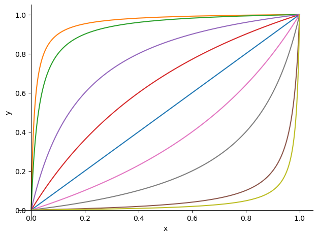
We can use this result to visualize more contract curves under different parameters

# Plot a range of αs and βs
params = [{α: 0.5, β: 0.5}, 
          {α: 0.1, β: 0.9},
          {α: 0.1, β: 0.8},
          {α: 0.8, β: 0.9},
          {α: 0.4, β: 0.8}, 
          {α: 0.8, β: 0.1},
          {α: 0.9, β: 0.8},
          {α: 0.8, β: 0.4},
          {α: 0.9, β: 0.1}]

p = plot(xlabel='x', ylabel='y', show=False)

for param in params:
    p_add = plot(sol.subs(param), (x, 0, 1), 
                 show=False)
    p.append(p_add[0])
p.show()

_images/9688629890c94fdbf3f49860309a9797d6c97f9a5d909720f4be66465360dfc8.png

We invite you to play with the parameters and see how the contract curves change and think about the following two questions:

Can you think of a way to draw the same graph using numpy?
How difficult will it be to write a numpy implementation?

15.7. Exercises #

Exercise 15.1

L’Hôpital’s rule states that for two functions \(f(x)\) and \(g(x)\), if \(\lim_{x \to a} f(x) = \lim_{x \to a} g(x) = 0\) or \(\pm \infty\), then

\[ \lim_{x \to a} \frac{f(x)}{g(x)} = \lim_{x \to a} \frac{f'(x)}{g'(x)} \]

Use SymPy to verify L’Hôpital’s rule for the following functions

\[ f(x) = \frac{y^x - 1}{x} \]

as \(x\) approaches to \(0\)

Solution to Exercise 15.1

Let’s define the function first

f_upper = y**x - 1
f_lower = x
f = f_upper/f_lower
f

\[\displaystyle \frac{y^{x} - 1}{x}\]

Sympy is smart enough to solve this limit

lim = limit(f, x, 0)
lim

\[\displaystyle \log{\left(y \right)}\]

We compare the result suggested by L’Hôpital’s rule

lim = limit(diff(f_upper, x)/
            diff(f_lower, x), x, 0)
lim

\[\displaystyle \log{\left(y \right)}\]

Exercise 15.2

Maximum likelihood estimation (MLE) is a method to estimate the parameters of a statistical model.

It usually involves maximizing a log-likelihood function and solving the first-order derivative.

The binomial distribution is given by

\[ f(x; n, θ) = \frac{n!}{x!(n-x)!}θ^x(1-θ)^{n-x} \]

where \(n\) is the number of trials and \(x\) is the number of successes.

Assume we observed a series of binary outcomes with \(x\) successes out of \(n\) trials.

Compute the MLE of \(θ\) using SymPy

Solution to Exercise 15.2

First, we define the binomial distribution

n, x, θ = symbols('n x θ')

binomial_factor = (factorial(n)) / (factorial(x)*factorial(n-r))
binomial_factor

\[\displaystyle \frac{n!}{x! \left(n - r\right)!}\]

bino_dist = binomial_factor * ((θ**x)*(1-θ)**(n-x))
bino_dist

\[\displaystyle \frac{θ^{x} \left(1 - θ\right)^{n - x} n!}{x! \left(n - r\right)!}\]

Now we compute the log-likelihood function and solve for the result

log_bino_dist = log(bino_dist)

log_bino_diff = simplify(diff(log_bino_dist, θ))
log_bino_diff

\[\displaystyle θ^{- x - 1} \left(1 - θ\right)^{- n + x - 1} \left(x θ^{x} \left(1 - θ\right)^{n - x + 1} - θ^{x + 1} \left(1 - θ\right)^{n - x} \left(n - x\right)\right)\]

solve(Eq(log_bino_diff, 0), θ)[0]

\[\displaystyle \frac{x}{n}\]