4. Functions

Contents

• Functions

  • Overview

  • Function Basics

  • Defining Functions

  • Applications

  • Recursive Function Calls (Advanced)

  • Exercises

  • Advanced Exercises

4.1. Overview

Functions are an extremely useful construct provided by almost all programming.

We have already met several functions, such as

• the sqrt() function from NumPy and

• the built-in print() function

In this lecture we’ll

1. treat functions systematically and cover syntax and use-cases, and

2. learn to do is build our own user-defined functions.

We will use the following imports.

import numpy as np
import matplotlib.pyplot as plt

4.2. Function Basics

A function is a named section of a program that implements a specific task.

Many functions exist already and we can use them as is.

First we review these functions and then discuss how we can build our own.

4.2.1. Built-In Functions

Python has a number of built-in functions that are available without import.

We have already met some

max(19, 20)

20

print('foobar')

foobar

str(22)

'22'

type(22)

int

The full list of Python built-ins is here.

4.2.2. Third Party Functions

If the built-in functions don’t cover what we need, we either need to import functions or create our own.

Examples of importing and using functions were given in the previous lecture

Here’s another one, which tests whether a given year is a leap year:

import calendar
calendar.isleap(2024)

True

4.3. Defining Functions

In many instances it’s useful to be able to define our own functions.

Let’s start by discussing how it’s done.

4.3.1. Basic Syntax

Here’s a very simple Python function, that implements the mathematical function \(f(x) = 2 x + 1\)

def f(x):
    return 2 * x + 1

Now that we’ve defined this function, let’s call it and check whether it does what we expect:

f(1)   

3

f(10)

21

Here’s a longer function, that computes the absolute value of a given number.

(Such a function already exists as a built-in, but let’s write our own for the exercise.)

def new_abs_function(x):
    if x < 0:
        abs_value = -x
    else:
        abs_value = x
    return abs_value

Let’s review the syntax here.

• def is a Python keyword used to start function definitions.

• def new_abs_function(x): indicates that the function is called new_abs_function and that it has a single argument x.

• The indented code is a code block called the function body.

• The return keyword indicates that abs_value is the object that should be returned to the calling code.

This whole function definition is read by the Python interpreter and stored in memory.

Let’s call it to check that it works:

print(new_abs_function(3))
print(new_abs_function(-3))

3
3

Note that a function can have arbitrarily many return statements (including zero).

Execution of the function terminates when the first return is hit, allowing code like the following example

def f(x):
    if x < 0:
        return 'negative'
    return 'nonnegative'

(Writing functions with multiple return statements is typically discouraged, as it can make logic hard to follow.)

Functions without a return statement automatically return the special Python object None.

4.3.2. Keyword Arguments

In a previous lecture, you came across the statement

plt.plot(x, 'b-', label="white noise")

In this call to Matplotlib’s plot function, notice that the last argument is passed in name=argument syntax.

This is called a keyword argument, with label being the keyword.

Non-keyword arguments are called positional arguments, since their meaning is determined by order

• plot(x, 'b-') differs from plot('b-', x)

Keyword arguments are particularly useful when a function has a lot of arguments, in which case it’s hard to remember the right order.

You can adopt keyword arguments in user-defined functions with no difficulty.

The next example illustrates the syntax

def f(x, a=1, b=1):
    return a + b * x

The keyword argument values we supplied in the definition of f become the default values

f(2)

3

They can be modified as follows

f(2, a=4, b=5)

14

4.3.3. The Flexibility of Python Functions

As we discussed in the previous lecture, Python functions are very flexible.

In particular

• Any number of functions can be defined in a given file.

• Functions can be (and often are) defined inside other functions.

• Any object can be passed to a function as an argument, including other functions.

• A function can return any kind of object, including functions.

We will give examples of how straightforward it is to pass a function to a function in the following sections.

4.3.4. One-Line Functions: lambda

The lambda keyword is used to create simple functions on one line.

For example, the definitions

def f(x):
    return x**3

and

f = lambda x: x**3

are entirely equivalent.

To see why lambda is useful, suppose that we want to calculate \(\int_0^2 x^3 dx\) (and have forgotten our high-school calculus).

The SciPy library has a function called quad that will do this calculation for us.

The syntax of the quad function is quad(f, a, b) where f is a function and a and b are numbers.

To create the function \(f(x) = x^3\) we can use lambda as follows

from scipy.integrate import quad

quad(lambda x: x**3, 0, 2)

(4.0, 4.440892098500626e-14)

Here the function created by lambda is said to be anonymous because it was never given a name.

4.3.5. Why Write Functions?

User-defined functions are important for improving the clarity of your code by

• separating different strands of logic

• facilitating code reuse

(Writing the same thing twice is almost always a bad idea)

We will say more about this later.

4.4. Applications

4.4.1. Random Draws

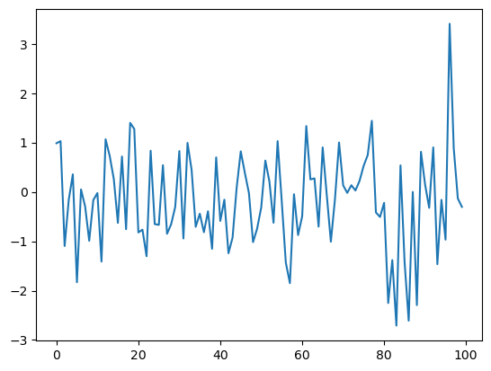
Consider again this code from the previous lecture

ts_length = 100
ϵ_values = []   # empty list

for i in range(ts_length):
    e = np.random.randn()
    ϵ_values.append(e)

plt.plot(ϵ_values)
plt.show()

We will break this program into two parts:

1. A user-defined function that generates a list of random variables.

2. The main part of the program that

   1. calls this function to get data

   2. plots the data

This is accomplished in the next program

def generate_data(n):
    ϵ_values = []
    for i in range(n):
        e = np.random.randn()
        ϵ_values.append(e)
    return ϵ_values

data = generate_data(100)
plt.plot(data)
plt.show()

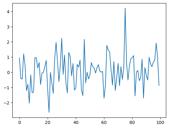
When the interpreter gets to the expression generate_data(100), it executes the function body with n set equal to 100.

The net result is that the name data is bound to the list ϵ_values returned by the function.

4.4.2. Adding Conditions

Our function generate_data() is rather limited.

Let’s make it slightly more useful by giving it the ability to return either standard normals or uniform random variables on \((0, 1)\) as required.

This is achieved in the next piece of code.

def generate_data(n, generator_type):
    ϵ_values = []
    for i in range(n):
        if generator_type == 'U':
            e = np.random.uniform(0, 1)
        else:
            e = np.random.randn()
        ϵ_values.append(e)
    return ϵ_values

data = generate_data(100, 'U')
plt.plot(data)
plt.show()

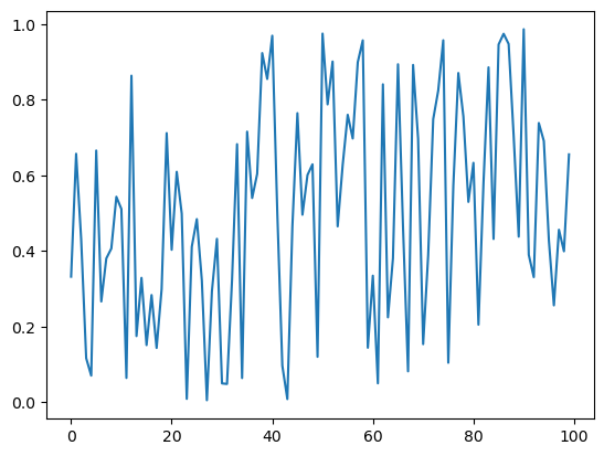
Hopefully, the syntax of the if/else clause is self-explanatory, with indentation again delimiting the extent of the code blocks.

Notes

• We are passing the argument U as a string, which is why we write it as 'U'.

• Notice that equality is tested with the == syntax, not =.

  • For example, the statement a = 10 assigns the name a to the value 10.

  • The expression a == 10 evaluates to either True or False, depending on the value of a.

Now, there are several ways that we can simplify the code above.

For example, we can get rid of the conditionals all together by just passing the desired generator type as a function.

To understand this, consider the following version.

def generate_data(n, generator_type):
    ϵ_values = []
    for i in range(n):
        e = generator_type()
        ϵ_values.append(e)
    return ϵ_values

data = generate_data(100, np.random.uniform)
plt.plot(data)
plt.show()

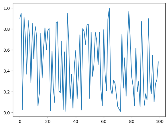
Now, when we call the function generate_data(), we pass np.random.uniform as the second argument.

This object is a function.

When the function call generate_data(100, np.random.uniform) is executed, Python runs the function code block with n equal to 100 and the name generator_type “bound” to the function np.random.uniform.

• While these lines are executed, the names generator_type and np.random.uniform are “synonyms”, and can be used in identical ways.

This principle works more generally—for example, consider the following piece of code

max(7, 2, 4)   # max() is a built-in Python function

7

m = max
m(7, 2, 4)

7

Here we created another name for the built-in function max(), which could then be used in identical ways.

In the context of our program, the ability to bind new names to functions means that there is no problem passing a function as an argument to another function—as we did above.

4.5. Recursive Function Calls (Advanced)

This is an advanced topic that you should feel free to skip.

At the same time, it’s a neat idea that you should learn it at some stage of your programming career.

Basically, a recursive function is a function that calls itself.

For example, consider the problem of computing \(x_t\) for some t when

(4.1)\[x_{t+1} = 2 x_t, \quad x_0 = 1\]

Obviously the answer is \(2^t\).

We can compute this easily enough with a loop

def x_loop(t):
    x = 1
    for i in range(t):
        x = 2 * x
    return x

We can also use a recursive solution, as follows

def x(t):
    if t == 0:
        return 1
    else:
        return 2 * x(t-1)

What happens here is that each successive call uses it’s own frame in the stack

• a frame is where the local variables of a given function call are held

• stack is memory used to process function calls

  • a First In Last Out (FILO) queue

This example is somewhat contrived, since the first (iterative) solution would usually be preferred to the recursive solution.

We’ll meet less contrived applications of recursion later on.

4.6. Exercises

Exercise 4.1

Recall that \(n!\) is read as “\(n\) factorial” and defined as \(n! = n \times (n - 1) \times \cdots \times 2 \times 1\).

We will only consider \(n\) as a positive integer here.

There are functions to compute this in various modules, but let’s write our own version as an exercise.

In particular, write a function factorial such that factorial(n) returns \(n!\) for any positive integer \(n\).

Solution to Exercise 4.1

Here’s one solution:

def factorial(n):
    k = 1
    for i in range(n):
        k = k * (i + 1)
    return k

factorial(4)

24

Exercise 4.2

The binomial random variable \(Y \sim Bin(n, p)\) represents the number of successes in \(n\) binary trials, where each trial succeeds with probability \(p\).

Without any import besides from numpy.random import uniform, write a function binomial_rv such that binomial_rv(n, p) generates one draw of \(Y\).

Hint

If \(U\) is uniform on \((0, 1)\) and \(p \in (0,1)\), then the expression U < p evaluates to True with probability \(p\).

Solution to Exercise 4.2

Here is one solution:

from numpy.random import uniform

def binomial_rv(n, p):
    count = 0
    for i in range(n):
        U = uniform()
        if U < p:
            count = count + 1    # Or count += 1
    return count

binomial_rv(10, 0.5)

3

Exercise 4.3

First, write a function that returns one realization of the following random device

1. Flip an unbiased coin 10 times.

2. If a head occurs k or more times consecutively within this sequence at least once, pay one dollar.

3. If not, pay nothing.

Second, write another function that does the same task except that the second rule of the above random device becomes

• If a head occurs k or more times within this sequence, pay one dollar.

Use no import besides from numpy.random import uniform.

Solution to Exercise 4.3

Here’s a function for the first random device.

from numpy.random import uniform

def draw(k):  # pays if k consecutive successes in a sequence

    payoff = 0
    count = 0

    for i in range(10):
        U = uniform()
        count = count + 1 if U < 0.5 else 0
        print(count)    # print counts for clarity
        if count == k:
            payoff = 1

    return payoff

draw(3)

0
1
0
0
0
0
1
2
3
4

1

Here’s another function for the second random device.

def draw_new(k):  # pays if k successes in a sequence

    payoff = 0
    count = 0

    for i in range(10):
        U = uniform()
        count = count + ( 1 if U < 0.5 else 0 )
        print(count)
        if count == k:
            payoff = 1

    return payoff

draw_new(3)

0
0
0
0
1
2
2
2
2
2

0

4.7. Advanced Exercises

In the following exercises, we will write recursive functions together.

Exercise 4.4

The Fibonacci numbers are defined by

(4.2)\[x_{t+1} = x_t + x_{t-1}, \quad x_0 = 0, \; x_1 = 1\]

The first few numbers in the sequence are \(0, 1, 1, 2, 3, 5, 8, 13, 21, 34, 55\).

Write a function to recursively compute the \(t\)-th Fibonacci number for any \(t\).

Solution to Exercise 4.4

Here’s the standard solution

def x(t):
    if t == 0:
        return 0
    if t == 1:
        return 1
    else:
        return x(t-1) + x(t-2)

Let’s test it

print([x(i) for i in range(10)])

[0, 1, 1, 2, 3, 5, 8, 13, 21, 34]

Exercise 4.5

Rewrite the function factorial() in from Exercise 1 using recursion.

Solution to Exercise 4.5

Here’s the standard solution

def recursion_factorial(n):
   if n == 1:
       return n
   else:
       return n * recursion_factorial(n-1)

Let’s test it

print([recursion_factorial(i) for i in range(1, 10)])

[1, 2, 6, 24, 120, 720, 5040, 40320, 362880]