17. Pandas#
In addition to what’s in Anaconda, this lecture will need the following libraries:
!pip install --upgrade wbgapi
!pip install --upgrade yfinance
17.1. Overview#
Pandas is a package of fast, efficient data analysis tools for Python.
Its popularity has surged in recent years, coincident with the rise of fields such as data science and machine learning.
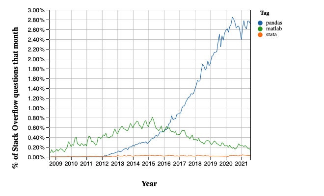
Here’s a popularity comparison over time against Matlab and STATA courtesy of Stack Overflow Trends
Just as NumPy provides the basic array data type plus core array operations, pandas
defines fundamental structures for working with data and
endows them with methods that facilitate operations such as
reading in data
adjusting indices
working with dates and time series
sorting, grouping, re-ordering and general data munging [1]
dealing with missing values, etc., etc.
More sophisticated statistical functionality is left to other packages, such as statsmodels and scikit-learn, which are built on top of pandas.
This lecture will provide a basic introduction to pandas.
Throughout the lecture, we will assume that the following imports have taken place
import pandas as pd
import numpy as np
import matplotlib.pyplot as plt
import requests
Two important data types defined by pandas are Series and DataFrame.
You can think of a Series as a “column” of data, such as a collection of observations on a single variable.
A DataFrame is a two-dimensional object for storing related columns of data.
17.2. Series#
Let’s start with Series.
We begin by creating a series of four random observations
s = pd.Series(np.random.randn(4), name='daily returns')
s
0    1.378496
1    0.515538
2    0.361642
3   -0.752114
Name: daily returns, dtype: float64
Here you can imagine the indices 0, 1, 2, 3 as indexing four listed
companies, and the values being daily returns on their shares.
Pandas Series are built on top of NumPy arrays and support many similar
operations
s * 100
0    137.849585
1     51.553786
2     36.164188
3    -75.211411
Name: daily returns, dtype: float64
np.abs(s)
0    1.378496
1    0.515538
2    0.361642
3    0.752114
Name: daily returns, dtype: float64
But Series provide more than NumPy arrays.
Not only do they have some additional (statistically oriented) methods
s.describe()
count    4.000000
mean     0.375890
std      0.875084
min     -0.752114
25%      0.083203
50%      0.438590
75%      0.731277
max      1.378496
Name: daily returns, dtype: float64
But their indices are more flexible
s.index = ['AMZN', 'AAPL', 'MSFT', 'GOOG']
s
AMZN    1.378496
AAPL    0.515538
MSFT    0.361642
GOOG   -0.752114
Name: daily returns, dtype: float64
Viewed in this way, Series are like fast, efficient Python dictionaries
(with the restriction that the items in the dictionary all have the same
type—in this case, floats).
In fact, you can use much of the same syntax as Python dictionaries
s['AMZN']
np.float64(1.37849585043469)
s['AMZN'] = 0
s
AMZN    0.000000
AAPL    0.515538
MSFT    0.361642
GOOG   -0.752114
Name: daily returns, dtype: float64
'AAPL' in s
True
17.3. DataFrames#
While a Series is a single column of data, a DataFrame is several columns, one for each variable.
In essence, a DataFrame in pandas is analogous to a (highly optimized) Excel spreadsheet.
Thus, it is a powerful tool for representing and analyzing data that are naturally organized into rows and columns, often with descriptive indexes for individual rows and individual columns.
Let’s look at an example that reads data from the CSV file pandas/data/test_pwt.csv, which is taken from the Penn World Tables.
The dataset contains the following indicators
Variable Name |
Description |
|---|---|
POP |
Population (in thousands) |
XRAT |
Exchange Rate to US Dollar |
tcgdp |
Total PPP Converted GDP (in million international dollar) |
cc |
Consumption Share of PPP Converted GDP Per Capita (%) |
cg |
Government Consumption Share of PPP Converted GDP Per Capita (%) |
We’ll read this in from a URL using the pandas function read_csv.
df = pd.read_csv('https://raw.githubusercontent.com/QuantEcon/lecture-python-programming/main/lectures/_static/lecture_specific/pandas/data/test_pwt.csv')
type(df)
pandas.core.frame.DataFrame
Here’s the content of test_pwt.csv
df
| country | country isocode | year | POP | XRAT | tcgdp | cc | cg | |
|---|---|---|---|---|---|---|---|---|
| 0 | Argentina | ARG | 2000 | 37335.653 | 0.999500 | 2.950722e+05 | 75.716805 | 5.578804 |
| 1 | Australia | AUS | 2000 | 19053.186 | 1.724830 | 5.418047e+05 | 67.759026 | 6.720098 |
| 2 | India | IND | 2000 | 1006300.297 | 44.941600 | 1.728144e+06 | 64.575551 | 14.072206 |
| 3 | Israel | ISR | 2000 | 6114.570 | 4.077330 | 1.292539e+05 | 64.436451 | 10.266688 |
| 4 | Malawi | MWI | 2000 | 11801.505 | 59.543808 | 5.026222e+03 | 74.707624 | 11.658954 |
| 5 | South Africa | ZAF | 2000 | 45064.098 | 6.939830 | 2.272424e+05 | 72.718710 | 5.726546 |
| 6 | United States | USA | 2000 | 282171.957 | 1.000000 | 9.898700e+06 | 72.347054 | 6.032454 |
| 7 | Uruguay | URY | 2000 | 3219.793 | 12.099592 | 2.525596e+04 | 78.978740 | 5.108068 |
17.3.1. Select Data by Position#
In practice, one thing that we do all the time is to find, select and work with a subset of the data of our interests.
We can select particular rows using standard Python array slicing notation
df[2:5]
| country | country isocode | year | POP | XRAT | tcgdp | cc | cg | |
|---|---|---|---|---|---|---|---|---|
| 2 | India | IND | 2000 | 1006300.297 | 44.941600 | 1.728144e+06 | 64.575551 | 14.072206 |
| 3 | Israel | ISR | 2000 | 6114.570 | 4.077330 | 1.292539e+05 | 64.436451 | 10.266688 |
| 4 | Malawi | MWI | 2000 | 11801.505 | 59.543808 | 5.026222e+03 | 74.707624 | 11.658954 |
To select columns, we can pass a list containing the names of the desired columns represented as strings
df[['country', 'tcgdp']]
| country | tcgdp | |
|---|---|---|
| 0 | Argentina | 2.950722e+05 |
| 1 | Australia | 5.418047e+05 |
| 2 | India | 1.728144e+06 |
| 3 | Israel | 1.292539e+05 |
| 4 | Malawi | 5.026222e+03 |
| 5 | South Africa | 2.272424e+05 |
| 6 | United States | 9.898700e+06 |
| 7 | Uruguay | 2.525596e+04 |
To select both rows and columns using integers, the iloc attribute should be used with the format .iloc[rows, columns].
df.iloc[2:5, 0:4]
| country | country isocode | year | POP | |
|---|---|---|---|---|
| 2 | India | IND | 2000 | 1006300.297 |
| 3 | Israel | ISR | 2000 | 6114.570 |
| 4 | Malawi | MWI | 2000 | 11801.505 |
To select rows and columns using a mixture of integers and labels, the loc attribute can be used in a similar way
df.loc[df.index[2:5], ['country', 'tcgdp']]
| country | tcgdp | |
|---|---|---|
| 2 | India | 1.728144e+06 |
| 3 | Israel | 1.292539e+05 |
| 4 | Malawi | 5.026222e+03 |
17.3.2. Select Data by Conditions#
Instead of indexing rows and columns using integers and names, we can also obtain a sub-dataframe of our interests that satisfies certain (potentially complicated) conditions.
This section demonstrates various ways to do that.
The most straightforward way is with the [] operator.
df[df.POP >= 20000]
| country | country isocode | year | POP | XRAT | tcgdp | cc | cg | |
|---|---|---|---|---|---|---|---|---|
| 0 | Argentina | ARG | 2000 | 37335.653 | 0.99950 | 2.950722e+05 | 75.716805 | 5.578804 |
| 2 | India | IND | 2000 | 1006300.297 | 44.94160 | 1.728144e+06 | 64.575551 | 14.072206 |
| 5 | South Africa | ZAF | 2000 | 45064.098 | 6.93983 | 2.272424e+05 | 72.718710 | 5.726546 |
| 6 | United States | USA | 2000 | 282171.957 | 1.00000 | 9.898700e+06 | 72.347054 | 6.032454 |
To understand what is going on here, notice that df.POP >= 20000 returns a series of boolean values.
df.POP >= 20000
0     True
1    False
2     True
3    False
4    False
5     True
6     True
7    False
Name: POP, dtype: bool
In this case, df[___] takes a series of boolean values and only returns rows with the True values.
Take one more example,
df[(df.country.isin(['Argentina', 'India', 'South Africa'])) & (df.POP > 40000)]
| country | country isocode | year | POP | XRAT | tcgdp | cc | cg | |
|---|---|---|---|---|---|---|---|---|
| 2 | India | IND | 2000 | 1006300.297 | 44.94160 | 1.728144e+06 | 64.575551 | 14.072206 |
| 5 | South Africa | ZAF | 2000 | 45064.098 | 6.93983 | 2.272424e+05 | 72.718710 | 5.726546 |
However, there is another way of doing the same thing, which can be slightly faster for large dataframes, with more natural syntax.
# the above is equivalent to
df.query("POP >= 20000")
| country | country isocode | year | POP | XRAT | tcgdp | cc | cg | |
|---|---|---|---|---|---|---|---|---|
| 0 | Argentina | ARG | 2000 | 37335.653 | 0.99950 | 2.950722e+05 | 75.716805 | 5.578804 |
| 2 | India | IND | 2000 | 1006300.297 | 44.94160 | 1.728144e+06 | 64.575551 | 14.072206 |
| 5 | South Africa | ZAF | 2000 | 45064.098 | 6.93983 | 2.272424e+05 | 72.718710 | 5.726546 |
| 6 | United States | USA | 2000 | 282171.957 | 1.00000 | 9.898700e+06 | 72.347054 | 6.032454 |
df.query("country in ['Argentina', 'India', 'South Africa'] and POP > 40000")
| country | country isocode | year | POP | XRAT | tcgdp | cc | cg | |
|---|---|---|---|---|---|---|---|---|
| 2 | India | IND | 2000 | 1006300.297 | 44.94160 | 1.728144e+06 | 64.575551 | 14.072206 |
| 5 | South Africa | ZAF | 2000 | 45064.098 | 6.93983 | 2.272424e+05 | 72.718710 | 5.726546 |
We can also allow arithmetic operations between different columns.
df[(df.cc + df.cg >= 80) & (df.POP <= 20000)]
| country | country isocode | year | POP | XRAT | tcgdp | cc | cg | |
|---|---|---|---|---|---|---|---|---|
| 4 | Malawi | MWI | 2000 | 11801.505 | 59.543808 | 5026.221784 | 74.707624 | 11.658954 |
| 7 | Uruguay | URY | 2000 | 3219.793 | 12.099592 | 25255.961693 | 78.978740 | 5.108068 |
# the above is equivalent to
df.query("cc + cg >= 80 & POP <= 20000")
| country | country isocode | year | POP | XRAT | tcgdp | cc | cg | |
|---|---|---|---|---|---|---|---|---|
| 4 | Malawi | MWI | 2000 | 11801.505 | 59.543808 | 5026.221784 | 74.707624 | 11.658954 |
| 7 | Uruguay | URY | 2000 | 3219.793 | 12.099592 | 25255.961693 | 78.978740 | 5.108068 |
For example, we can use the conditioning to select the country with the largest household consumption - gdp share cc.
df.loc[df.cc == max(df.cc)]
| country | country isocode | year | POP | XRAT | tcgdp | cc | cg | |
|---|---|---|---|---|---|---|---|---|
| 7 | Uruguay | URY | 2000 | 3219.793 | 12.099592 | 25255.961693 | 78.97874 | 5.108068 |
When we only want to look at certain columns of a selected sub-dataframe, we can use the above conditions with the .loc[__ , __] command.
The first argument takes the condition, while the second argument takes a list of columns we want to return.
df.loc[(df.cc + df.cg >= 80) & (df.POP <= 20000), ['country', 'year', 'POP']]
| country | year | POP | |
|---|---|---|---|
| 4 | Malawi | 2000 | 11801.505 |
| 7 | Uruguay | 2000 | 3219.793 |
Application: Subsetting Dataframe
Real-world datasets can be enormous.
It is sometimes desirable to work with a subset of data to enhance computational efficiency and reduce redundancy.
Let’s imagine that we’re only interested in the population (POP) and total GDP (tcgdp).
One way to strip the data frame df down to only these variables is to overwrite the dataframe using the selection method described above
df_subset = df[['country', 'POP', 'tcgdp']]
df_subset
| country | POP | tcgdp | |
|---|---|---|---|
| 0 | Argentina | 37335.653 | 2.950722e+05 |
| 1 | Australia | 19053.186 | 5.418047e+05 |
| 2 | India | 1006300.297 | 1.728144e+06 |
| 3 | Israel | 6114.570 | 1.292539e+05 |
| 4 | Malawi | 11801.505 | 5.026222e+03 |
| 5 | South Africa | 45064.098 | 2.272424e+05 |
| 6 | United States | 282171.957 | 9.898700e+06 |
| 7 | Uruguay | 3219.793 | 2.525596e+04 |
We can then save the smaller dataset for further analysis.
df_subset.to_csv('pwt_subset.csv', index=False)
17.3.3. Apply Method#
Another widely used Pandas method is df.apply().
It applies a function to each row/column and returns a series.
This function can be some built-in functions like the max function, a lambda function, or a user-defined function.
Here is an example using the max function
df[['year', 'POP', 'XRAT', 'tcgdp', 'cc', 'cg']].apply(max)
year     2.000000e+03
POP      1.006300e+06
XRAT     5.954381e+01
tcgdp    9.898700e+06
cc       7.897874e+01
cg       1.407221e+01
dtype: float64
This line of code applies the max function to all selected columns.
lambda function is often used with df.apply() method
A trivial example is to return itself for each row in the dataframe
df.apply(lambda row: row, axis=1)
| country | country isocode | year | POP | XRAT | tcgdp | cc | cg | |
|---|---|---|---|---|---|---|---|---|
| 0 | Argentina | ARG | 2000 | 37335.653 | 0.999500 | 2.950722e+05 | 75.716805 | 5.578804 |
| 1 | Australia | AUS | 2000 | 19053.186 | 1.724830 | 5.418047e+05 | 67.759026 | 6.720098 |
| 2 | India | IND | 2000 | 1006300.297 | 44.941600 | 1.728144e+06 | 64.575551 | 14.072206 |
| 3 | Israel | ISR | 2000 | 6114.570 | 4.077330 | 1.292539e+05 | 64.436451 | 10.266688 |
| 4 | Malawi | MWI | 2000 | 11801.505 | 59.543808 | 5.026222e+03 | 74.707624 | 11.658954 |
| 5 | South Africa | ZAF | 2000 | 45064.098 | 6.939830 | 2.272424e+05 | 72.718710 | 5.726546 |
| 6 | United States | USA | 2000 | 282171.957 | 1.000000 | 9.898700e+06 | 72.347054 | 6.032454 |
| 7 | Uruguay | URY | 2000 | 3219.793 | 12.099592 | 2.525596e+04 | 78.978740 | 5.108068 |
Note
For the .apply() method
axis = 0 – apply function to each column (variables)
axis = 1 – apply function to each row (observations)
axis = 0 is the default parameter
We can use it together with .loc[] to do some more advanced selection.
complexCondition = df.apply(
    lambda row: row.POP > 40000 if row.country in ['Argentina', 'India', 'South Africa'] else row.POP < 20000,
    axis=1), ['country', 'year', 'POP', 'XRAT', 'tcgdp']
df.apply() here returns a series of boolean values rows that satisfies the condition specified in the if-else statement.
In addition, it also defines a subset of variables of interest.
complexCondition
(0    False
 1     True
 2     True
 3     True
 4     True
 5     True
 6    False
 7     True
 dtype: bool,
 ['country', 'year', 'POP', 'XRAT', 'tcgdp'])
When we apply this condition to the dataframe, the result will be
df.loc[complexCondition]
| country | year | POP | XRAT | tcgdp | |
|---|---|---|---|---|---|
| 1 | Australia | 2000 | 19053.186 | 1.724830 | 5.418047e+05 |
| 2 | India | 2000 | 1006300.297 | 44.941600 | 1.728144e+06 |
| 3 | Israel | 2000 | 6114.570 | 4.077330 | 1.292539e+05 |
| 4 | Malawi | 2000 | 11801.505 | 59.543808 | 5.026222e+03 |
| 5 | South Africa | 2000 | 45064.098 | 6.939830 | 2.272424e+05 |
| 7 | Uruguay | 2000 | 3219.793 | 12.099592 | 2.525596e+04 |
17.3.4. Make Changes in DataFrames#
The ability to make changes in dataframes is important to generate a clean dataset for future analysis.
1. We can use df.where() conveniently to “keep” the rows we have selected and replace the rest rows with any other values
df.where(df.POP >= 20000, False)
| country | country isocode | year | POP | XRAT | tcgdp | cc | cg | |
|---|---|---|---|---|---|---|---|---|
| 0 | Argentina | ARG | 2000 | 37335.653 | 0.9995 | 295072.21869 | 75.716805 | 5.578804 |
| 1 | False | False | False | False | False | False | False | False |
| 2 | India | IND | 2000 | 1006300.297 | 44.9416 | 1728144.3748 | 64.575551 | 14.072206 |
| 3 | False | False | False | False | False | False | False | False |
| 4 | False | False | False | False | False | False | False | False |
| 5 | South Africa | ZAF | 2000 | 45064.098 | 6.93983 | 227242.36949 | 72.71871 | 5.726546 |
| 6 | United States | USA | 2000 | 282171.957 | 1.0 | 9898700.0 | 72.347054 | 6.032454 |
| 7 | False | False | False | False | False | False | False | False |
2. We can simply use .loc[] to specify the column that we want to modify, and assign values
df.loc[df.cg == max(df.cg), 'cg'] = np.nan
df
| country | country isocode | year | POP | XRAT | tcgdp | cc | cg | |
|---|---|---|---|---|---|---|---|---|
| 0 | Argentina | ARG | 2000 | 37335.653 | 0.999500 | 2.950722e+05 | 75.716805 | 5.578804 |
| 1 | Australia | AUS | 2000 | 19053.186 | 1.724830 | 5.418047e+05 | 67.759026 | 6.720098 |
| 2 | India | IND | 2000 | 1006300.297 | 44.941600 | 1.728144e+06 | 64.575551 | NaN |
| 3 | Israel | ISR | 2000 | 6114.570 | 4.077330 | 1.292539e+05 | 64.436451 | 10.266688 |
| 4 | Malawi | MWI | 2000 | 11801.505 | 59.543808 | 5.026222e+03 | 74.707624 | 11.658954 |
| 5 | South Africa | ZAF | 2000 | 45064.098 | 6.939830 | 2.272424e+05 | 72.718710 | 5.726546 |
| 6 | United States | USA | 2000 | 282171.957 | 1.000000 | 9.898700e+06 | 72.347054 | 6.032454 |
| 7 | Uruguay | URY | 2000 | 3219.793 | 12.099592 | 2.525596e+04 | 78.978740 | 5.108068 |
3. We can use the .apply() method to modify rows/columns as a whole
def update_row(row):
    # modify POP
    row.POP = np.nan if row.POP<= 10000 else row.POP

    # modify XRAT
    row.XRAT = row.XRAT / 10
    return row

df.apply(update_row, axis=1)
| country | country isocode | year | POP | XRAT | tcgdp | cc | cg | |
|---|---|---|---|---|---|---|---|---|
| 0 | Argentina | ARG | 2000 | 37335.653 | 0.099950 | 2.950722e+05 | 75.716805 | 5.578804 |
| 1 | Australia | AUS | 2000 | 19053.186 | 0.172483 | 5.418047e+05 | 67.759026 | 6.720098 |
| 2 | India | IND | 2000 | 1006300.297 | 4.494160 | 1.728144e+06 | 64.575551 | NaN |
| 3 | Israel | ISR | 2000 | NaN | 0.407733 | 1.292539e+05 | 64.436451 | 10.266688 |
| 4 | Malawi | MWI | 2000 | 11801.505 | 5.954381 | 5.026222e+03 | 74.707624 | 11.658954 |
| 5 | South Africa | ZAF | 2000 | 45064.098 | 0.693983 | 2.272424e+05 | 72.718710 | 5.726546 |
| 6 | United States | USA | 2000 | 282171.957 | 0.100000 | 9.898700e+06 | 72.347054 | 6.032454 |
| 7 | Uruguay | URY | 2000 | NaN | 1.209959 | 2.525596e+04 | 78.978740 | 5.108068 |
4. We can use the .map() method to modify all individual entries in the dataframe altogether.
# Round all decimal numbers to 2 decimal places
df.map(lambda x : round(x,2) if type(x)!=str else x)
| country | country isocode | year | POP | XRAT | tcgdp | cc | cg | |
|---|---|---|---|---|---|---|---|---|
| 0 | Argentina | ARG | 2000 | 37335.65 | 1.00 | 295072.22 | 75.72 | 5.58 |
| 1 | Australia | AUS | 2000 | 19053.19 | 1.72 | 541804.65 | 67.76 | 6.72 |
| 2 | India | IND | 2000 | 1006300.30 | 44.94 | 1728144.37 | 64.58 | NaN |
| 3 | Israel | ISR | 2000 | 6114.57 | 4.08 | 129253.89 | 64.44 | 10.27 |
| 4 | Malawi | MWI | 2000 | 11801.50 | 59.54 | 5026.22 | 74.71 | 11.66 |
| 5 | South Africa | ZAF | 2000 | 45064.10 | 6.94 | 227242.37 | 72.72 | 5.73 |
| 6 | United States | USA | 2000 | 282171.96 | 1.00 | 9898700.00 | 72.35 | 6.03 |
| 7 | Uruguay | URY | 2000 | 3219.79 | 12.10 | 25255.96 | 78.98 | 5.11 |
Application: Missing Value Imputation
Replacing missing values is an important step in data munging.
Let’s randomly insert some NaN values
for idx in list(zip([0, 3, 5, 6], [3, 4, 6, 2])):
    df.iloc[idx] = np.nan

df
| country | country isocode | year | POP | XRAT | tcgdp | cc | cg | |
|---|---|---|---|---|---|---|---|---|
| 0 | Argentina | ARG | 2000.0 | NaN | 0.999500 | 2.950722e+05 | 75.716805 | 5.578804 |
| 1 | Australia | AUS | 2000.0 | 19053.186 | 1.724830 | 5.418047e+05 | 67.759026 | 6.720098 |
| 2 | India | IND | 2000.0 | 1006300.297 | 44.941600 | 1.728144e+06 | 64.575551 | NaN |
| 3 | Israel | ISR | 2000.0 | 6114.570 | NaN | 1.292539e+05 | 64.436451 | 10.266688 |
| 4 | Malawi | MWI | 2000.0 | 11801.505 | 59.543808 | 5.026222e+03 | 74.707624 | 11.658954 |
| 5 | South Africa | ZAF | 2000.0 | 45064.098 | 6.939830 | 2.272424e+05 | NaN | 5.726546 |
| 6 | United States | USA | NaN | 282171.957 | 1.000000 | 9.898700e+06 | 72.347054 | 6.032454 |
| 7 | Uruguay | URY | 2000.0 | 3219.793 | 12.099592 | 2.525596e+04 | 78.978740 | 5.108068 |
The zip() function here creates pairs of values from the two lists (i.e. [0,3], [3,4] …)
We can use the .map() method again to replace all missing values with 0
# replace all NaN values by 0
def replace_nan(x):
    if type(x)!=str:
        return  0 if np.isnan(x) else x
    else:
        return x

df.map(replace_nan)
| country | country isocode | year | POP | XRAT | tcgdp | cc | cg | |
|---|---|---|---|---|---|---|---|---|
| 0 | Argentina | ARG | 2000.0 | 0.000 | 0.999500 | 2.950722e+05 | 75.716805 | 5.578804 |
| 1 | Australia | AUS | 2000.0 | 19053.186 | 1.724830 | 5.418047e+05 | 67.759026 | 6.720098 |
| 2 | India | IND | 2000.0 | 1006300.297 | 44.941600 | 1.728144e+06 | 64.575551 | 0.000000 |
| 3 | Israel | ISR | 2000.0 | 6114.570 | 0.000000 | 1.292539e+05 | 64.436451 | 10.266688 |
| 4 | Malawi | MWI | 2000.0 | 11801.505 | 59.543808 | 5.026222e+03 | 74.707624 | 11.658954 |
| 5 | South Africa | ZAF | 2000.0 | 45064.098 | 6.939830 | 2.272424e+05 | 0.000000 | 5.726546 |
| 6 | United States | USA | 0.0 | 282171.957 | 1.000000 | 9.898700e+06 | 72.347054 | 6.032454 |
| 7 | Uruguay | URY | 2000.0 | 3219.793 | 12.099592 | 2.525596e+04 | 78.978740 | 5.108068 |
Pandas also provides us with convenient methods to replace missing values.
For example, single imputation using variable means can be easily done in pandas
df = df.fillna(df.iloc[:,2:8].mean())
df
| country | country isocode | year | POP | XRAT | tcgdp | cc | cg | |
|---|---|---|---|---|---|---|---|---|
| 0 | Argentina | ARG | 2000.0 | 1.962465e+05 | 0.999500 | 2.950722e+05 | 75.716805 | 5.578804 |
| 1 | Australia | AUS | 2000.0 | 1.905319e+04 | 1.724830 | 5.418047e+05 | 67.759026 | 6.720098 |
| 2 | India | IND | 2000.0 | 1.006300e+06 | 44.941600 | 1.728144e+06 | 64.575551 | 7.298802 |
| 3 | Israel | ISR | 2000.0 | 6.114570e+03 | 18.178451 | 1.292539e+05 | 64.436451 | 10.266688 |
| 4 | Malawi | MWI | 2000.0 | 1.180150e+04 | 59.543808 | 5.026222e+03 | 74.707624 | 11.658954 |
| 5 | South Africa | ZAF | 2000.0 | 4.506410e+04 | 6.939830 | 2.272424e+05 | 71.217322 | 5.726546 |
| 6 | United States | USA | 2000.0 | 2.821720e+05 | 1.000000 | 9.898700e+06 | 72.347054 | 6.032454 |
| 7 | Uruguay | URY | 2000.0 | 3.219793e+03 | 12.099592 | 2.525596e+04 | 78.978740 | 5.108068 |
Missing value imputation is a big area in data science involving various machine learning techniques.
There are also more advanced tools in python to impute missing values.
17.3.5. Standardization and Visualization#
Let’s imagine that we’re only interested in the population (POP) and total GDP (tcgdp).
One way to strip the data frame df down to only these variables is to overwrite the dataframe using the selection method described above
df = df[['country', 'POP', 'tcgdp']]
df
| country | POP | tcgdp | |
|---|---|---|---|
| 0 | Argentina | 1.962465e+05 | 2.950722e+05 |
| 1 | Australia | 1.905319e+04 | 5.418047e+05 |
| 2 | India | 1.006300e+06 | 1.728144e+06 |
| 3 | Israel | 6.114570e+03 | 1.292539e+05 |
| 4 | Malawi | 1.180150e+04 | 5.026222e+03 |
| 5 | South Africa | 4.506410e+04 | 2.272424e+05 |
| 6 | United States | 2.821720e+05 | 9.898700e+06 |
| 7 | Uruguay | 3.219793e+03 | 2.525596e+04 |
Here the index 0, 1,..., 7 is redundant because we can use the country names as an index.
To do this, we set the index to be the country variable in the dataframe
df = df.set_index('country')
df
| POP | tcgdp | |
|---|---|---|
| country | ||
| Argentina | 1.962465e+05 | 2.950722e+05 |
| Australia | 1.905319e+04 | 5.418047e+05 |
| India | 1.006300e+06 | 1.728144e+06 |
| Israel | 6.114570e+03 | 1.292539e+05 |
| Malawi | 1.180150e+04 | 5.026222e+03 |
| South Africa | 4.506410e+04 | 2.272424e+05 |
| United States | 2.821720e+05 | 9.898700e+06 |
| Uruguay | 3.219793e+03 | 2.525596e+04 |
Let’s give the columns slightly better names
df.columns = 'population', 'total GDP'
df
| population | total GDP | |
|---|---|---|
| country | ||
| Argentina | 1.962465e+05 | 2.950722e+05 |
| Australia | 1.905319e+04 | 5.418047e+05 |
| India | 1.006300e+06 | 1.728144e+06 |
| Israel | 6.114570e+03 | 1.292539e+05 |
| Malawi | 1.180150e+04 | 5.026222e+03 |
| South Africa | 4.506410e+04 | 2.272424e+05 |
| United States | 2.821720e+05 | 9.898700e+06 |
| Uruguay | 3.219793e+03 | 2.525596e+04 |
The population variable is in thousands, let’s revert to single units
df['population'] = df['population'] * 1e3
df
| population | total GDP | |
|---|---|---|
| country | ||
| Argentina | 1.962465e+08 | 2.950722e+05 |
| Australia | 1.905319e+07 | 5.418047e+05 |
| India | 1.006300e+09 | 1.728144e+06 |
| Israel | 6.114570e+06 | 1.292539e+05 |
| Malawi | 1.180150e+07 | 5.026222e+03 |
| South Africa | 4.506410e+07 | 2.272424e+05 |
| United States | 2.821720e+08 | 9.898700e+06 |
| Uruguay | 3.219793e+06 | 2.525596e+04 |
Next, we’re going to add a column showing real GDP per capita, multiplying by 1,000,000 as we go because total GDP is in millions
df['GDP percap'] = df['total GDP'] * 1e6 / df['population']
df
| population | total GDP | GDP percap | |
|---|---|---|---|
| country | |||
| Argentina | 1.962465e+08 | 2.950722e+05 | 1503.579625 |
| Australia | 1.905319e+07 | 5.418047e+05 | 28436.433261 |
| India | 1.006300e+09 | 1.728144e+06 | 1717.324719 |
| Israel | 6.114570e+06 | 1.292539e+05 | 21138.672749 |
| Malawi | 1.180150e+07 | 5.026222e+03 | 425.896679 |
| South Africa | 4.506410e+07 | 2.272424e+05 | 5042.647686 |
| United States | 2.821720e+08 | 9.898700e+06 | 35080.381854 |
| Uruguay | 3.219793e+06 | 2.525596e+04 | 7843.970620 |
One of the nice things about pandas DataFrame and Series objects is that they have methods for plotting and visualization that work through Matplotlib.
For example, we can easily generate a bar plot of GDP per capita
ax = df['GDP percap'].plot(kind='bar')
ax.set_xlabel('country', fontsize=12)
ax.set_ylabel('GDP per capita', fontsize=12)
plt.show()
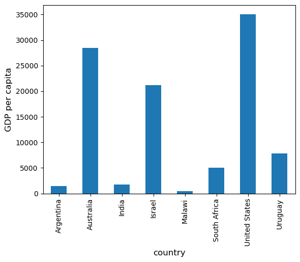
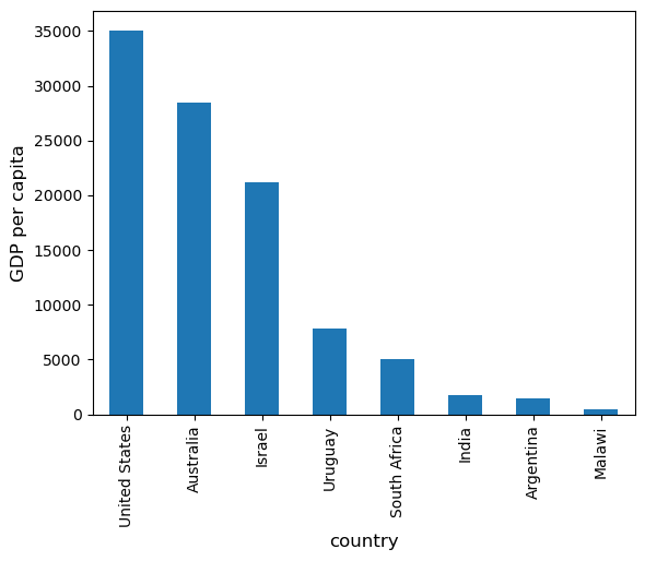
At the moment the data frame is ordered alphabetically on the countries—let’s change it to GDP per capita
df = df.sort_values(by='GDP percap', ascending=False)
df
| population | total GDP | GDP percap | |
|---|---|---|---|
| country | |||
| United States | 2.821720e+08 | 9.898700e+06 | 35080.381854 |
| Australia | 1.905319e+07 | 5.418047e+05 | 28436.433261 |
| Israel | 6.114570e+06 | 1.292539e+05 | 21138.672749 |
| Uruguay | 3.219793e+06 | 2.525596e+04 | 7843.970620 |
| South Africa | 4.506410e+07 | 2.272424e+05 | 5042.647686 |
| India | 1.006300e+09 | 1.728144e+06 | 1717.324719 |
| Argentina | 1.962465e+08 | 2.950722e+05 | 1503.579625 |
| Malawi | 1.180150e+07 | 5.026222e+03 | 425.896679 |
Plotting as before now yields
ax = df['GDP percap'].plot(kind='bar')
ax.set_xlabel('country', fontsize=12)
ax.set_ylabel('GDP per capita', fontsize=12)
plt.show()
17.4. On-Line Data Sources#
Python makes it straightforward to query online databases programmatically.
An important database for economists is FRED — a vast collection of time series data maintained by the St. Louis Fed.
For example, suppose that we are interested in the unemployment rate.
(To download the data as a csv, click on the top right Download and select the CSV (data) option).
Alternatively, we can access the CSV file from within a Python program.
This can be done with a variety of methods.
We start with a relatively low-level method and then return to pandas.
17.4.1. Accessing Data with requests#
One option is to use requests, a standard Python library for requesting data over the Internet.
To begin, try the following code on your computer
r = requests.get('https://fred.stlouisfed.org/graph/fredgraph.csv?bgcolor=%23e1e9f0&chart_type=line&drp=0&fo=open%20sans&graph_bgcolor=%23ffffff&height=450&mode=fred&recession_bars=on&txtcolor=%23444444&ts=12&tts=12&width=1318&nt=0&thu=0&trc=0&show_legend=yes&show_axis_titles=yes&show_tooltip=yes&id=UNRATE&scale=left&cosd=1948-01-01&coed=2024-06-01&line_color=%234572a7&link_values=false&line_style=solid&mark_type=none&mw=3&lw=2&ost=-99999&oet=99999&mma=0&fml=a&fq=Monthly&fam=avg&fgst=lin&fgsnd=2020-02-01&line_index=1&transformation=lin&vintage_date=2024-07-29&revision_date=2024-07-29&nd=1948-01-01')
If there’s no error message, then the call has succeeded.
If you do get an error, then there are two likely causes
You are not connected to the Internet — hopefully, this isn’t the case.
Your machine is accessing the Internet through a proxy server, and Python isn’t aware of this.
In the second case, you can either
switch to another machine
solve your proxy problem by reading the documentation
Assuming that all is working, you can now proceed to use the source object returned by the call requests.get('https://research.stlouisfed.org/fred2/series/UNRATE/downloaddata/UNRATE.csv')
url = 'https://fred.stlouisfed.org/graph/fredgraph.csv?bgcolor=%23e1e9f0&chart_type=line&drp=0&fo=open%20sans&graph_bgcolor=%23ffffff&height=450&mode=fred&recession_bars=on&txtcolor=%23444444&ts=12&tts=12&width=1318&nt=0&thu=0&trc=0&show_legend=yes&show_axis_titles=yes&show_tooltip=yes&id=UNRATE&scale=left&cosd=1948-01-01&coed=2024-06-01&line_color=%234572a7&link_values=false&line_style=solid&mark_type=none&mw=3&lw=2&ost=-99999&oet=99999&mma=0&fml=a&fq=Monthly&fam=avg&fgst=lin&fgsnd=2020-02-01&line_index=1&transformation=lin&vintage_date=2024-07-29&revision_date=2024-07-29&nd=1948-01-01'
source = requests.get(url).content.decode().split("\n")
source[0]
'observation_date,UNRATE'
source[1]
'1948-01-01,3.4'
source[2]
'1948-02-01,3.8'
We could now write some additional code to parse this text and store it as an array.
But this is unnecessary — pandas’ read_csv function can handle the task for us.
We use parse_dates=True so that pandas recognizes our dates column, allowing for simple date filtering
data = pd.read_csv(url, index_col=0, parse_dates=True)
The data has been read into a pandas DataFrame called data that we can now manipulate in the usual way
type(data)
pandas.core.frame.DataFrame
data.head() # A useful method to get a quick look at a data frame
| UNRATE | |
|---|---|
| observation_date | |
| 1948-01-01 | 3.4 |
| 1948-02-01 | 3.8 |
| 1948-03-01 | 4.0 |
| 1948-04-01 | 3.9 |
| 1948-05-01 | 3.5 |
pd.set_option('display.precision', 1)
data.describe()  # Your output might differ slightly
| UNRATE | |
|---|---|
| count | 918.0 |
| mean | 5.7 |
| std | 1.7 |
| min | 2.5 |
| 25% | 4.4 |
| 50% | 5.5 |
| 75% | 6.7 |
| max | 14.8 |
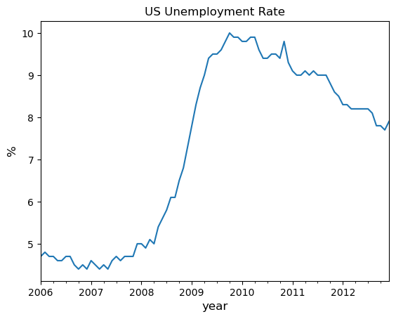
We can also plot the unemployment rate from 2006 to 2012 as follows
ax = data['2006':'2012'].plot(title='US Unemployment Rate', legend=False)
ax.set_xlabel('year', fontsize=12)
ax.set_ylabel('%', fontsize=12)
plt.show()
Note that pandas offers many other file type alternatives.
Pandas has a wide variety of top-level methods that we can use to read, excel, json, parquet or plug straight into a database server.
17.4.2. Using wbgapi and yfinance to Access Data#
The wbgapi python library can be used to fetch data from the many databases published by the World Bank.
Note
You can find some useful information about the wbgapi package in this world bank blog post, in addition to this tutorial
We will also use yfinance to fetch data from Yahoo finance in the exercises.
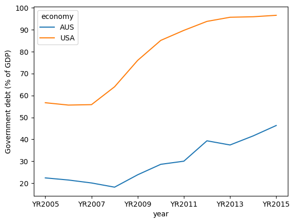
For now let’s work through one example of downloading and plotting data — this time from the World Bank.
The World Bank collects and organizes data on a huge range of indicators.
For example, here’s some data on government debt as a ratio to GDP.
The next code example fetches the data for you and plots time series for the US and Australia
import wbgapi as wb
wb.series.info('GC.DOD.TOTL.GD.ZS')
| id | value |
|---|---|
| GC.DOD.TOTL.GD.ZS | Central government debt, total (% of GDP) |
| 1 elements |
govt_debt = wb.data.DataFrame('GC.DOD.TOTL.GD.ZS', economy=['USA','AUS'], time=range(2005,2016))
govt_debt = govt_debt.T    # move years from columns to rows for plotting
govt_debt.plot(xlabel='year', ylabel='Government debt (% of GDP)');
17.5. Exercises#
Exercise 17.1
With these imports:
import datetime as dt
import yfinance as yf
Write a program to calculate the percentage price change over 2021 for the following shares:
ticker_list = {'INTC': 'Intel',
               'MSFT': 'Microsoft',
               'IBM': 'IBM',
               'BHP': 'BHP',
               'TM': 'Toyota',
               'AAPL': 'Apple',
               'AMZN': 'Amazon',
               'C': 'Citigroup',
               'QCOM': 'Qualcomm',
               'KO': 'Coca-Cola',
               'GOOG': 'Google'}
Here’s the first part of the program
def read_data(ticker_list,
          start=dt.datetime(2021, 1, 1),
          end=dt.datetime(2021, 12, 31)):
    """
    This function reads in closing price data from Yahoo
    for each tick in the ticker_list.
    """
    ticker = pd.DataFrame()

    for tick in ticker_list:
        stock = yf.Ticker(tick)
        prices = stock.history(start=start, end=end)

        # Change the index to date-only
        prices.index = pd.to_datetime(prices.index.date)

        closing_prices = prices['Close']
        ticker[tick] = closing_prices

    return ticker

ticker = read_data(ticker_list)
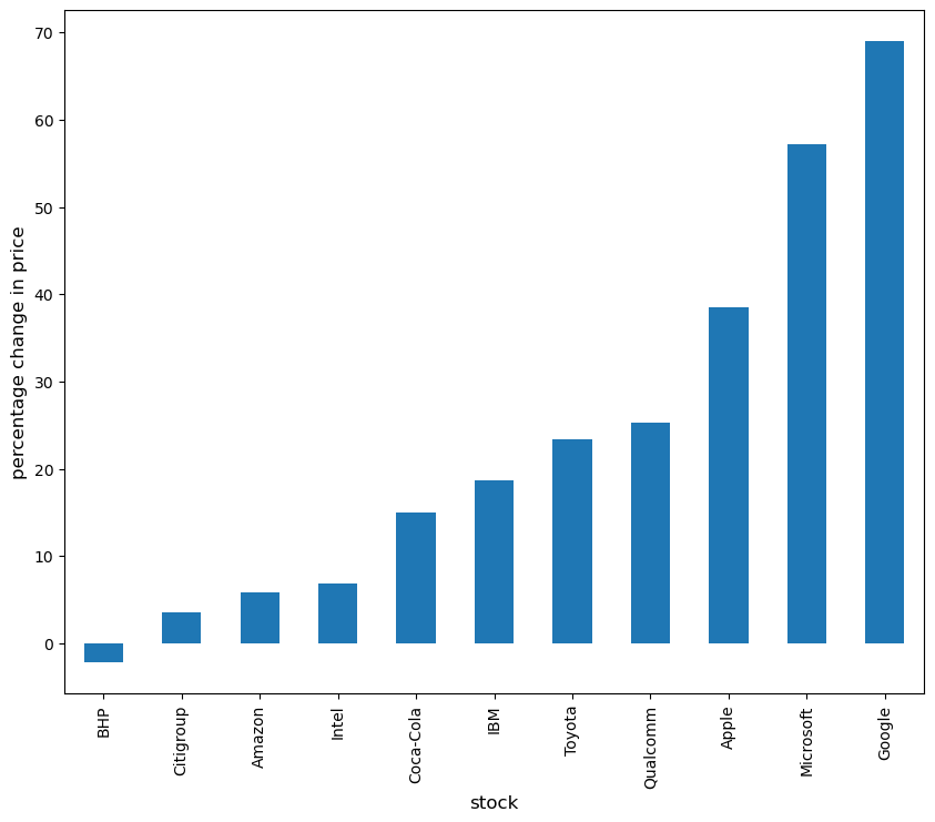
Complete the program to plot the result as a bar graph like this one:
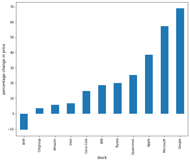
Solution
There are a few ways to approach this problem using Pandas to calculate the percentage change.
First, you can extract the data and perform the calculation such as:
p1 = ticker.iloc[0]    #Get the first set of prices as a Series
p2 = ticker.iloc[-1]   #Get the last set of prices as a Series
price_change = (p2 - p1) / p1 * 100
price_change
INTC     6.9
MSFT    57.2
IBM     18.7
BHP     -2.2
TM      23.4
AAPL    38.6
AMZN     5.8
C        3.6
QCOM    25.3
KO      14.9
GOOG    69.0
dtype: float64
Alternatively you can use an inbuilt method pct_change and configure it to
perform the correct calculation using periods argument.
change = ticker.pct_change(periods=len(ticker)-1, axis='rows')*100
price_change = change.iloc[-1]
price_change
INTC     6.9
MSFT    57.2
IBM     18.7
BHP     -2.2
TM      23.4
AAPL    38.6
AMZN     5.8
C        3.6
QCOM    25.3
KO      14.9
GOOG    69.0
Name: 2021-12-30 00:00:00, dtype: float64
Then to plot the chart
price_change.sort_values(inplace=True)
price_change.rename(index=ticker_list, inplace=True)
/tmp/ipykernel_3084/1503263560.py:1: SettingWithCopyWarning:
A value is trying to be set on a copy of a slice from a DataFrame

See the caveats in the documentation: https://pandas.pydata.org/pandas-docs/stable/user_guide/indexing.html#returning-a-view-versus-a-copy
  price_change.sort_values(inplace=True)
/tmp/ipykernel_3084/1503263560.py:2: SettingWithCopyWarning:
A value is trying to be set on a copy of a slice from a DataFrame

See the caveats in the documentation: https://pandas.pydata.org/pandas-docs/stable/user_guide/indexing.html#returning-a-view-versus-a-copy
  price_change.rename(index=ticker_list, inplace=True)
fig, ax = plt.subplots(figsize=(10,8))
ax.set_xlabel('stock', fontsize=12)
ax.set_ylabel('percentage change in price', fontsize=12)
price_change.plot(kind='bar', ax=ax)
plt.show()
Exercise 17.2
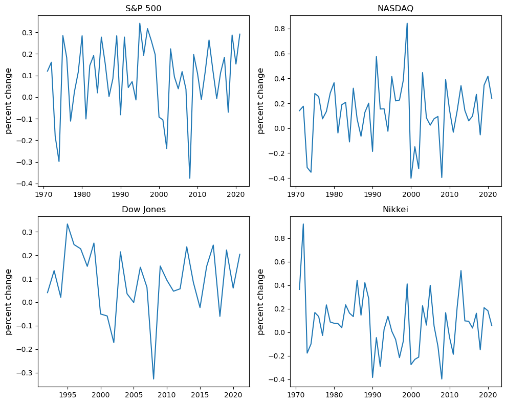
Using the method read_data introduced in Exercise 17.1, write a program to obtain year-on-year percentage change for the following indices:
indices_list = {'^GSPC': 'S&P 500',
               '^IXIC': 'NASDAQ',
               '^DJI': 'Dow Jones',
               '^N225': 'Nikkei'}
Complete the program to show summary statistics and plot the result as a time series graph like this one:
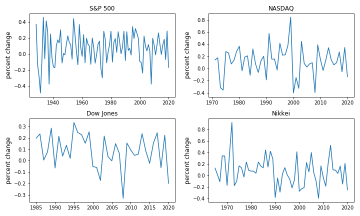
Solution
Following the work you did in Exercise 17.1, you can query the data using read_data by updating the start and end dates accordingly.
indices_data = read_data(
        indices_list,
        start=dt.datetime(1971, 1, 1),  #Common Start Date
        end=dt.datetime(2021, 12, 31)
)
Then, extract the first and last set of prices per year as DataFrames and calculate the yearly returns such as:
yearly_returns = pd.DataFrame()

for index, name in indices_list.items():
    p1 = indices_data.groupby(indices_data.index.year)[index].first()  # Get the first set of returns as a DataFrame
    p2 = indices_data.groupby(indices_data.index.year)[index].last()   # Get the last set of returns as a DataFrame
    returns = (p2 - p1) / p1
    yearly_returns[name] = returns

yearly_returns
| S&P 500 | NASDAQ | Dow Jones | Nikkei | |
|---|---|---|---|---|
| 1971 | 1.2e-01 | 1.4e-01 | NaN | 3.6e-01 |
| 1972 | 1.6e-01 | 1.8e-01 | NaN | 9.2e-01 |
| 1973 | -1.8e-01 | -3.2e-01 | NaN | -1.8e-01 |
| 1974 | -3.0e-01 | -3.5e-01 | NaN | -9.9e-02 |
| 1975 | 2.8e-01 | 2.8e-01 | NaN | 1.7e-01 |
| 1976 | 1.8e-01 | 2.5e-01 | NaN | 1.3e-01 |
| 1977 | -1.1e-01 | 7.5e-02 | NaN | -2.7e-02 |
| 1978 | 2.4e-02 | 1.3e-01 | NaN | 2.3e-01 |
| 1979 | 1.2e-01 | 2.8e-01 | NaN | 8.7e-02 |
| 1980 | 2.8e-01 | 3.7e-01 | NaN | 7.7e-02 |
| 1981 | -1.0e-01 | -3.8e-02 | NaN | 7.4e-02 |
| 1982 | 1.5e-01 | 1.9e-01 | NaN | 3.9e-02 |
| 1983 | 1.9e-01 | 2.1e-01 | NaN | 2.3e-01 |
| 1984 | 2.0e-02 | -1.1e-01 | NaN | 1.6e-01 |
| 1985 | 2.8e-01 | 3.2e-01 | NaN | 1.3e-01 |
| 1986 | 1.6e-01 | 7.3e-02 | NaN | 4.4e-01 |
| 1987 | 2.6e-03 | -6.4e-02 | NaN | 1.5e-01 |
| 1988 | 8.5e-02 | 1.3e-01 | NaN | 4.2e-01 |
| 1989 | 2.8e-01 | 2.0e-01 | NaN | 2.9e-01 |
| 1990 | -8.2e-02 | -1.9e-01 | NaN | -3.8e-01 |
| 1991 | 2.8e-01 | 5.8e-01 | NaN | -4.5e-02 |
| 1992 | 4.4e-02 | 1.5e-01 | 4.1e-02 | -2.9e-01 |
| 1993 | 7.1e-02 | 1.6e-01 | 1.3e-01 | 2.5e-02 |
| 1994 | -1.3e-02 | -2.4e-02 | 2.1e-02 | 1.4e-01 |
| 1995 | 3.4e-01 | 4.1e-01 | 3.3e-01 | 9.4e-03 |
| 1996 | 1.9e-01 | 2.2e-01 | 2.5e-01 | -6.1e-02 |
| 1997 | 3.2e-01 | 2.3e-01 | 2.3e-01 | -2.2e-01 |
| 1998 | 2.6e-01 | 3.9e-01 | 1.5e-01 | -7.5e-02 |
| 1999 | 2.0e-01 | 8.4e-01 | 2.5e-01 | 4.1e-01 |
| 2000 | -9.3e-02 | -4.0e-01 | -5.0e-02 | -2.7e-01 |
| 2001 | -1.1e-01 | -1.5e-01 | -5.9e-02 | -2.3e-01 |
| 2002 | -2.4e-01 | -3.3e-01 | -1.7e-01 | -2.1e-01 |
| 2003 | 2.2e-01 | 4.5e-01 | 2.1e-01 | 2.3e-01 |
| 2004 | 9.3e-02 | 8.4e-02 | 3.6e-02 | 6.1e-02 |
| 2005 | 3.8e-02 | 2.5e-02 | -1.1e-03 | 4.0e-01 |
| 2006 | 1.2e-01 | 7.6e-02 | 1.5e-01 | 5.3e-02 |
| 2007 | 3.7e-02 | 9.5e-02 | 6.3e-02 | -1.2e-01 |
| 2008 | -3.8e-01 | -4.0e-01 | -3.3e-01 | -4.0e-01 |
| 2009 | 2.0e-01 | 3.9e-01 | 1.5e-01 | 1.7e-01 |
| 2010 | 1.1e-01 | 1.5e-01 | 9.4e-02 | -4.0e-02 |
| 2011 | -1.1e-02 | -3.2e-02 | 4.7e-02 | -1.9e-01 |
| 2012 | 1.2e-01 | 1.4e-01 | 5.7e-02 | 2.1e-01 |
| 2013 | 2.6e-01 | 3.4e-01 | 2.4e-01 | 5.2e-01 |
| 2014 | 1.2e-01 | 1.4e-01 | 8.4e-02 | 9.7e-02 |
| 2015 | -6.9e-03 | 5.9e-02 | -2.3e-02 | 9.3e-02 |
| 2016 | 1.1e-01 | 9.8e-02 | 1.5e-01 | 3.6e-02 |
| 2017 | 1.8e-01 | 2.7e-01 | 2.4e-01 | 1.6e-01 |
| 2018 | -7.0e-02 | -5.3e-02 | -6.0e-02 | -1.5e-01 |
| 2019 | 2.9e-01 | 3.5e-01 | 2.2e-01 | 2.1e-01 |
| 2020 | 1.5e-01 | 4.2e-01 | 6.0e-02 | 1.8e-01 |
| 2021 | 2.9e-01 | 2.4e-01 | 2.0e-01 | 5.6e-02 |
Next, you can obtain summary statistics by using the method describe.
yearly_returns.describe()
| S&P 500 | NASDAQ | Dow Jones | Nikkei | |
|---|---|---|---|---|
| count | 5.1e+01 | 5.1e+01 | 3.0e+01 | 5.1e+01 |
| mean | 9.2e-02 | 1.3e-01 | 9.1e-02 | 7.9e-02 |
| std | 1.6e-01 | 2.5e-01 | 1.4e-01 | 2.4e-01 |
| min | -3.8e-01 | -4.0e-01 | -3.3e-01 | -4.0e-01 |
| 25% | -2.2e-03 | 1.6e-04 | 2.5e-02 | -6.8e-02 |
| 50% | 1.2e-01 | 1.4e-01 | 8.9e-02 | 7.7e-02 |
| 75% | 2.0e-01 | 2.8e-01 | 2.1e-01 | 2.0e-01 |
| max | 3.4e-01 | 8.4e-01 | 3.3e-01 | 9.2e-01 |
Then, to plot the chart
fig, axes = plt.subplots(2, 2, figsize=(10, 8))

for iter_, ax in enumerate(axes.flatten()):            # Flatten 2-D array to 1-D array
    index_name = yearly_returns.columns[iter_]         # Get index name per iteration
    ax.plot(yearly_returns[index_name])                # Plot pct change of yearly returns per index
    ax.set_ylabel("percent change", fontsize = 12)
    ax.set_title(index_name)

plt.tight_layout()