12. SciPy#
In addition to what’s in Anaconda, this lecture will need the following libraries:
!pip install --upgrade quantecon
We use the following imports.
import numpy as np
import quantecon as qe
12.1. Overview#
SciPy builds on top of NumPy to provide common tools for scientific programming such as
etc., etc
Like NumPy, SciPy is stable, mature and widely used.
Many SciPy routines are thin wrappers around industry-standard Fortran libraries such as LAPACK, BLAS, etc.
It’s not really necessary to “learn” SciPy as a whole.
A more common approach is to get some idea of what’s in the library and then look up documentation as required.
In this lecture, we aim only to highlight some useful parts of the package.
12.2. SciPy versus NumPy#
SciPy is a package that contains various tools that are built on top of NumPy, using its array data type and related functionality.
Note
In older versions of SciPy (scipy < 0.15.1), importing the package would also import NumPy symbols into the global namespace, as can be seen from this excerpt the SciPy initialization file:
from numpy import *
from numpy.random import rand, randn
from numpy.fft import fft, ifft
from numpy.lib.scimath import *
However, it is better practice to use NumPy functionality explicitly.
import numpy as np

a = np.identity(3)
More recent versions of SciPy (1.15+) no longer automatically import NumPy symbols.
What is useful in SciPy is the functionality in its sub-packages
scipy.optimize,scipy.integrate,scipy.stats, etc.
Let’s explore some of the major sub-packages.
12.3. Statistics#
The scipy.stats subpackage supplies
numerous random variable objects (densities, cumulative distributions, random sampling, etc.)
some estimation procedures
some statistical tests
12.3.1. Random Variables and Distributions#
Recall that numpy.random provides tools for generating random variables
rng = np.random.default_rng()
rng.beta(5, 5, size=3)
array([0.58811869, 0.77705054, 0.52177983])
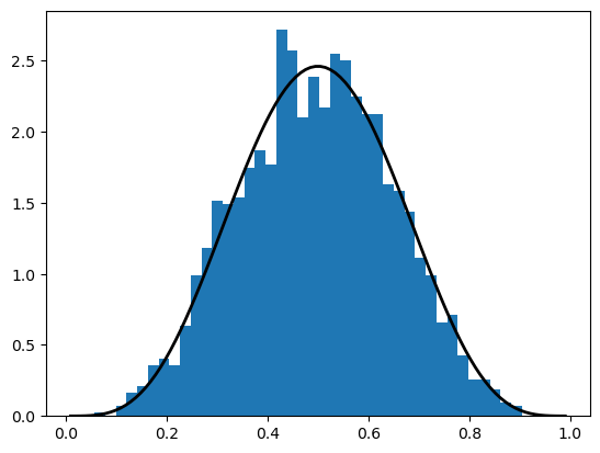
This generates a draw from the distribution with the density function below when a, b = 5, 5
Sometimes we need access to the density itself, or the cdf, the quantiles, etc.
For this, we can use scipy.stats, which provides all of this functionality as well as random number generation in a single consistent interface.
Here’s an example of usage
from scipy.stats import beta
import matplotlib.pyplot as plt

q = beta(5, 5)      # Beta(a, b), with a = b = 5
obs = q.rvs(2000)   # 2000 observations
grid = np.linspace(0.01, 0.99, 100)

fig, ax = plt.subplots()
ax.hist(obs, bins=40, density=True)
ax.plot(grid, q.pdf(grid), 'k-', linewidth=2)
plt.show()
The object q that represents the distribution has additional useful methods, including
q.cdf(0.4) # Cumulative distribution function
np.float64(0.26656768000000003)
q.ppf(0.8) # Quantile (inverse cdf) function
np.float64(0.6339134834642708)
q.mean()
np.float64(0.5)
The general syntax for creating these objects that represent distributions (of type rv_frozen) is
name = scipy.stats.distribution_name(shape_parameters, loc=c, scale=d)
Here distribution_name is one of the distribution names in scipy.stats.
The loc and scale parameters transform the original random variable
\(X\) into \(Y = c + d X\).
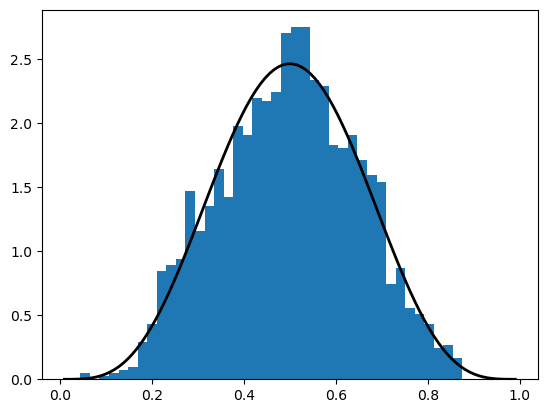
12.3.2. Alternative Syntax#
There is an alternative way of calling the methods described above.
For example, the code that generates the figure above can be replaced by
obs = beta.rvs(5, 5, size=2000)
grid = np.linspace(0.01, 0.99, 100)

fig, ax = plt.subplots()
ax.hist(obs, bins=40, density=True)
ax.plot(grid, beta.pdf(grid, 5, 5), 'k-', linewidth=2)
plt.show()
12.3.3. Other Goodies in scipy.stats#
There are a variety of statistical functions in scipy.stats.
For example, scipy.stats.linregress implements simple linear regression
from scipy.stats import linregress

x = rng.standard_normal(200)
y = 2 * x + 0.1 * rng.standard_normal(200)
gradient, intercept, r_value, p_value, std_err = linregress(x, y)
gradient, intercept
(np.float64(1.9961243825038208), np.float64(-0.009279782990134901))
To see the full list, consult the documentation.
12.4. Roots and Fixed Points#
A root or zero of a real function \(f\) on \([a,b]\) is an \(x \in [a, b]\) such that \(f(x)=0\).
For example, if we plot the function
with \(x \in [0,1]\) we get
f = lambda x: np.sin(4 * (x - 1/4)) + x + x**20 - 1
x = np.linspace(0, 1, 100)

fig, ax = plt.subplots()
ax.plot(x, f(x), label='$f(x)$')
ax.axhline(ls='--', c='k')
ax.set_xlabel('$x$', fontsize=12)
ax.set_ylabel('$f(x)$', fontsize=12)
ax.legend(fontsize=12)
plt.show()
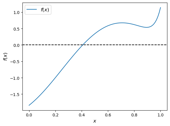
The unique root is approximately 0.408.
Let’s consider some numerical techniques for finding roots.
12.4.1. Bisection#
One of the most common algorithms for numerical root-finding is bisection.
To understand the idea, recall the well-known game where
Player A thinks of a secret number between 1 and 100
Player B asks if it’s less than 50
If yes, B asks if it’s less than 25
If no, B asks if it’s less than 75
And so on.
This is bisection.
Here’s a simplistic implementation of the algorithm in Python.
It works for all sufficiently well behaved increasing continuous functions with \(f(a) < 0 < f(b)\)
def bisect(f, a, b, tol=10e-5):
    """
    Implements the bisection root finding algorithm, assuming that f is a
    real-valued function on [a, b] satisfying f(a) < 0 < f(b).
    """
    lower, upper = a, b

    while upper - lower > tol:
        middle = 0.5 * (upper + lower)
        if f(middle) > 0:   # root is between lower and middle
            lower, upper = lower, middle
        else:               # root is between middle and upper
            lower, upper = middle, upper

    return 0.5 * (upper + lower)
Let’s test it using the function \(f\) defined in (12.2)
bisect(f, 0, 1)
0.408294677734375
Not surprisingly, SciPy provides its own bisection function.
Let’s test it using the same function \(f\) defined in (12.2)
from scipy.optimize import bisect

bisect(f, 0, 1)
0.4082935042806639
12.4.2. The Newton-Raphson Method#
Another very common root-finding algorithm is the Newton-Raphson method.
In SciPy this algorithm is implemented by scipy.optimize.newton.
Unlike bisection, the Newton-Raphson method uses local slope information in an attempt to increase the speed of convergence.
Let’s investigate this using the same function \(f\) defined above.
With a suitable initial condition for the search we get convergence:
from scipy.optimize import newton

newton(f, 0.2)   # Start the search at initial condition x = 0.2
np.float64(0.40829350427935673)
But other initial conditions lead to failure of convergence:
newton(f, 0.7) # Start the search at x = 0.7 instead
np.float64(0.7001700000000279)
12.4.3. Hybrid Methods#
A general principle of numerical methods is as follows:
If you have specific knowledge about a given problem, you might be able to exploit it to generate efficiency.
If not, then the choice of algorithm involves a trade-off between speed and robustness.
In practice, most default algorithms for root-finding, optimization and fixed points use hybrid methods.
These methods typically combine a fast method with a robust method in the following manner:
Attempt to use a fast method
Check diagnostics
If diagnostics are bad, then switch to a more robust algorithm
In scipy.optimize, the function brentq is such a hybrid method and a good default
from scipy.optimize import brentq

brentq(f, 0, 1)
0.40829350427936706
Here the correct solution is found and the speed is better than bisection:
with qe.Timer(unit="milliseconds"):
    brentq(f, 0, 1)
0.0398 ms elapsed
with qe.Timer(unit="milliseconds"):
    bisect(f, 0, 1)
0.0889 ms elapsed
12.4.4. Multivariate Root-Finding#
Use scipy.optimize.fsolve, a wrapper for a hybrid method in MINPACK.
See the documentation for details.
12.4.5. Fixed Points#
A fixed point of a real function \(f\) on \([a,b]\) is an \(x \in [a, b]\) such that \(f(x)=x\).
SciPy has a function for finding (scalar) fixed points too
from scipy.optimize import fixed_point

fixed_point(lambda x: x**2, 10.0)  # 10.0 is an initial guess
array(1.)
If you don’t get good results, you can always switch back to the brentq root finder, since
the fixed point of a function \(f\) is the root of \(g(x) := x - f(x)\).
12.5. Optimization#
Most numerical packages provide only functions for minimization.
Maximization can be performed by recalling that the maximizer of a function \(f\) on domain \(D\) is the minimizer of \(-f\) on \(D\).
Minimization is closely related to root-finding: For smooth functions, interior optima correspond to roots of the first derivative.
The speed/robustness trade-off described above is present with numerical optimization too.
Unless you have some prior information you can exploit, it’s usually best to use hybrid methods.
For constrained, univariate (i.e., scalar) minimization, a good hybrid option is fminbound
from scipy.optimize import fminbound

fminbound(lambda x: x**2, -1, 2)  # Search in [-1, 2]
np.float64(0.0)
12.5.1. Multivariate Optimization#
Multivariate local optimizers include minimize, fmin, fmin_powell, fmin_cg, fmin_bfgs, and fmin_ncg.
Constrained multivariate local optimizers include fmin_l_bfgs_b, fmin_tnc, fmin_cobyla.
See the documentation for details.
12.6. Integration#
Most numerical integration methods work by computing the integral of an approximating polynomial.
The resulting error depends on how well the polynomial fits the integrand, which in turn depends on how “regular” the integrand is.
In SciPy, the relevant module for numerical integration is scipy.integrate.
A good default for univariate integration is quad
from scipy.integrate import quad

integral, error = quad(lambda x: x**2, 0, 1)
integral
0.33333333333333337
In fact, quad is an interface to a very standard numerical integration routine in the Fortran library QUADPACK.
It uses Clenshaw-Curtis quadrature, based on expansion in terms of Chebychev polynomials.
There are other options for univariate integration—a useful one is fixed_quad, which is fast and hence works well inside for loops.
There are also functions for multivariate integration.
See the documentation for more details.
12.7. Linear Algebra#
We saw that NumPy provides a module for linear algebra called linalg.
SciPy also provides a module for linear algebra with the same name.
The latter is not an exact superset of the former, but overall it has more functionality.
We leave you to investigate the set of available routines.
12.8. Exercises#
The first few exercises concern pricing a European call option under the assumption of risk neutrality. The price satisfies
where
\(\beta\) is a discount factor,
\(n\) is the expiry date,
\(K\) is the strike price and
\(\{S_t\}\) is the price of the underlying asset at each time \(t\).
For example, if the call option is to buy stock in Amazon at strike price \(K\), the owner has the right (but not the obligation) to buy 1 share in Amazon at price \(K\) after \(n\) days.
The payoff is therefore \(\max\{S_n - K, 0\}\)
The price is the expectation of the payoff, discounted to current value.
Exercise 12.1
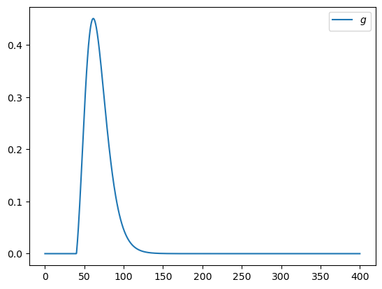
Suppose that \(S_n\) has the log-normal distribution with parameters \(\mu\) and \(\sigma\). Let \(f\) denote the density of this distribution. Then
Plot the function
over the interval \([0, 400]\) when μ, σ, β, n, K = 4, 0.25, 0.99, 10, 40.
Hint
From scipy.stats you can import lognorm and then use lognorm.pdf(x, σ, scale=np.exp(μ)) to get the density \(f\).
Solution
Here’s one possible solution
from scipy.integrate import quad
from scipy.stats import lognorm

μ, σ, β, n, K = 4, 0.25, 0.99, 10, 40

def g(x):
    return β**n * np.maximum(x - K, 0) * lognorm.pdf(x, σ, scale=np.exp(μ))

x_grid = np.linspace(0, 400, 1000)
y_grid = g(x_grid)

fig, ax = plt.subplots()
ax.plot(x_grid, y_grid, label="$g$")
ax.legend()
plt.show()
Exercise 12.2
In order to get the option price, compute the integral of this function numerically using quad from scipy.integrate.
Solution
P, error = quad(g, 0, 1_000)
print(f"The numerical integration based option price is {P:.3f}")
The numerical integration based option price is 15.188
Exercise 12.3
Try to get a similar result using Monte Carlo to compute the expectation term in the option price, rather than quad.
In particular, use the fact that if \(S_n^1, \ldots, S_n^M\) are independent draws from the lognormal distribution specified above, then, by the law of large numbers,
Set M = 10_000_000
Solution
Here is one solution:
rng = np.random.default_rng()
M = 10_000_000
S = np.exp(μ + σ * rng.standard_normal(M))
return_draws = np.maximum(S - K, 0)
P = β**n * np.mean(return_draws)
print(f"The Monte Carlo option price is {P:3f}")
The Monte Carlo option price is 15.187786
Exercise 12.4
In this lecture, we discussed the concept of recursive function calls.
Try to write a recursive implementation of the homemade bisection function described above.
Test it on the function (12.2).
Solution
Here’s a reasonable solution:
def bisect(f, a, b, tol=10e-5):
    """
    Implements the bisection root-finding algorithm, assuming that f is a
    real-valued function on [a, b] satisfying f(a) < 0 < f(b).
    """
    lower, upper = a, b
    if upper - lower < tol:
        return 0.5 * (upper + lower)
    else:
        middle = 0.5 * (upper + lower)
        print(f'Current mid point = {middle}')
        if f(middle) > 0:   # Implies root is between lower and middle
            return bisect(f, lower, middle)
        else:               # Implies root is between middle and upper
            return bisect(f, middle, upper)
We can test it as follows
f = lambda x: np.sin(4 * (x - 0.25)) + x + x**20 - 1
bisect(f, 0, 1)
Current mid point = 0.5
Current mid point = 0.25
Current mid point = 0.375
Current mid point = 0.4375
Current mid point = 0.40625
Current mid point = 0.421875
Current mid point = 0.4140625
Current mid point = 0.41015625
Current mid point = 0.408203125
Current mid point = 0.4091796875
Current mid point = 0.40869140625
Current mid point = 0.408447265625
Current mid point = 0.4083251953125
Current mid point = 0.40826416015625
0.408294677734375