14. JAX#
This lecture provides a short introduction to Google JAX.
GPU
This lecture was built using a machine with access to a GPU — although it will also run without one.
Google Colab has a free tier with GPUs that you can access as follows:
Click on the “play” icon top right
Select Colab
Set the runtime environment to include a GPU
JAX is a high-performance scientific computing library that provides
a NumPy-like interface that can automatically parallelize across CPUs and GPUs,
a just-in-time compiler for accelerating a large range of numerical operations, and
Increasingly, JAX also maintains and provides more specialized scientific computing routines, such as those originally found in SciPy.
In addition to what’s in Anaconda, this lecture will need the following libraries:
!pip install jax quantecon
We’ll use the following imports
import jax
import jax.numpy as jnp
import matplotlib.pyplot as plt
import numpy as np
import quantecon as qe
14.1. JAX as a NumPy Replacement#
Let’s look at the similarities and differences between JAX and NumPy.
14.1.1. Similarities#
Above we import jax.numpy as jnp, which provides a NumPy-like interface to
array operations.
One of the attractive features of JAX is that, whenever possible, this interface conform to the NumPy API.
As a result, we can often use JAX as a drop-in NumPy replacement.
Here are some standard array operations using jnp:
a = jnp.asarray((1.0, 3.2, -1.5))
print(a)
[ 1. 3.2 -1.5]
print(jnp.sum(a))
2.6999998
print(jnp.dot(a, a))
13.490001
It should be remembered, however, that the array object a is not a NumPy array:
a
Array([ 1. , 3.2, -1.5], dtype=float32)
type(a)
jaxlib._jax.ArrayImpl
Even scalar-valued maps on arrays return JAX arrays rather than scalars!
jnp.sum(a)
Array(2.6999998, dtype=float32)
14.1.2. Differences#
Let’s now look at some differences between JAX and NumPy array operations.
14.1.2.1. Speed!#
One major difference is that JAX is faster — and sometimes much faster.
To illustrate, suppose that we want to evaluate the cosine function at many points.
n = 50_000_000
x = np.linspace(0, 10, n)   # NumPy array
14.1.2.1.1. With NumPy#
Let’s try with NumPy
with qe.Timer():
    # First NumPy timing
    y = np.cos(x)
0.6838 seconds elapsed
And one more time.
with qe.Timer():
    # Second NumPy timing
    y = np.cos(x)
0.6844 seconds elapsed
Here
NumPy uses a pre-built binary for applying cosine to an array of floats
The binary runs on the local machine’s CPU
14.1.2.1.2. With JAX#
Now let’s try with JAX.
x = jnp.linspace(0, 10, n)
Let’s time the same procedure.
with qe.Timer():
    # First run
    y = jnp.cos(x)
    # Hold the interpreter until the array operation finishes
    y.block_until_ready()
0.0860 seconds elapsed
Note
Above, the block_until_ready method
holds the interpreter until the results of the computation are returned.
This is necessary for timing execution because JAX uses asynchronous dispatch, which
allows the Python interpreter to run ahead of numerical computations.
Now let’s time it again.
with qe.Timer():
    # Second run
    y = jnp.cos(x)
    # Hold interpreter
    y.block_until_ready()
0.0018 seconds elapsed
On a GPU, this code runs much faster than its NumPy equivalent.
Also, typically, the second run is faster than the first due to JIT compilation.
This is because even built in functions like jnp.cos are JIT-compiled — and the
first run includes compile time.
Why would JAX want to JIT-compile built in functions like jnp.cos instead of
just providing pre-compiled versions, like NumPy?
The reason is that the JIT compiler wants to specialize on the size of the array being used (as well as the data type).
The size matters for generating optimized code because efficient parallelization requires matching the size of the task to the available hardware.
14.1.2.2. Size Experiment#
We can verify the claim that JAX specializes on array size by changing the input size and watching the runtimes.
x = jnp.linspace(0, 10, n + 1)
with qe.Timer():
    # First run
    y = jnp.cos(x)
    # Hold interpreter
    y.block_until_ready()
0.0578 seconds elapsed
with qe.Timer():
    # Second run
    y = jnp.cos(x)
    # Hold interpreter
    y.block_until_ready()
0.0021 seconds elapsed
The run time increases and then falls again (this will be more obvious on the GPU).
This is in line with the discussion above – the first run after changing array size shows compilation overhead.
Further discussion of JIT compilation is provided below.
14.1.2.3. Precision#
Another difference between NumPy and JAX is that JAX uses 32 bit floats by default.
This is because JAX is often used for GPU computing, and most GPU computations use 32 bit floats.
Using 32 bit floats can lead to significant speed gains with small loss of precision.
However, for some calculations precision matters.
In these cases 64 bit floats can be enforced via the command
jax.config.update("jax_enable_x64", True)
Let’s check this works:
jnp.ones(3)
Array([1., 1., 1.], dtype=float64)
14.1.2.4. Immutability#
As a NumPy replacement, a more significant difference is that arrays are treated as immutable.
For example, with NumPy we can write
a = np.linspace(0, 1, 3)
a
array([0. , 0.5, 1. ])
and then mutate the data in memory:
a[0] = 1
a
array([1. , 0.5, 1. ])
In JAX this fails 😱.
a = jnp.linspace(0, 1, 3)
a
Array([0. , 0.5, 1. ], dtype=float64)
try:
    a[0] = 1
except Exception as e:
    print(e)
JAX arrays are immutable and do not support in-place item assignment. Instead of x[idx] = y, use x = x.at[idx].set(y) or another .at[] method: https://docs.jax.dev/en/latest/_autosummary/jax.numpy.ndarray.at.html
The designers of JAX chose to make arrays immutable because
JAX uses a functional programming style and
functional programming typically avoids mutable data
We discuss these ideas below.
14.1.2.5. A Workaround#
JAX does provide a direct alternative to in-place array modification
via the at method.
a = jnp.linspace(0, 1, 3)
Applying at[0].set(1) returns a new copy of a with the first element set to 1
a = a.at[0].set(1)
a
Array([1. , 0.5, 1. ], dtype=float64)
Obviously, there are downsides to using at:
The syntax is cumbersome and
we want to avoid creating fresh arrays in memory every time we change a single value!
Hence, for the most part, we try to avoid this syntax.
(Although it can in fact be efficient inside JIT-compiled functions – but let’s put this aside for now.)
14.2. Functional Programming#
From JAX’s documentation:
When walking about the countryside of Italy, the people will not hesitate to tell you that JAX has “una anima di pura programmazione funzionale”.
In other words, JAX assumes a functional programming style.
14.2.1. Pure functions#
The major implication is that JAX functions should be pure.
Pure functions have the following characteristics:
Deterministic
No side effects
Deterministic means
Same input \(\implies\) same output
Outputs do not depend on global state
In particular, pure functions will always return the same result if invoked with the same inputs.
No side effects means that the function
Won’t change global state
Won’t modify data passed to the function (immutable data)
14.2.2. Examples – Pure and Impure#
Here’s an example of a impure function
tax_rate = 0.1

def add_tax(prices):
    for i, price in enumerate(prices):
        prices[i] = price * (1 + tax_rate)

prices = [10.0, 20.0]
add_tax(prices)
prices
[11.0, 22.0]
This function fails to be pure because
side effects — it modifies the global variable
pricesnon-deterministic — a change to the global variable
tax_ratewill modify function outputs, even with the same input arrayprices.
Here’s a pure version
def add_tax_pure(prices, tax_rate):
    new_prices = [price * (1 + tax_rate) for price in prices]
    return new_prices

tax_rate = 0.1
prices = (10.0, 20.0)
after_tax_prices = add_tax_pure(prices, tax_rate)
after_tax_prices
[11.0, 22.0]
This is pure because
all dependencies explicit through function arguments
and doesn’t modify any external state
14.2.3. Why Functional Programming?#
At QuantEcon we love pure functions because they
Help testing: each function can operate in isolation
Promote deterministic behavior and hence reproducibility
Prevent bugs that arise from mutating shared state
The JAX compiler loves pure functions and functional programming because
Data dependencies are explicit, which helps with optimizing complex computations
Pure functions are easier to differentiate (autodiff)
Pure functions are easier to parallelize and optimize (don’t depend on shared mutable state)
Another way to think of this is as follows:
JAX represents functions as computational graphs, which are then compiled or transformed (e.g., differentiated)
These computational graphs describe how a given set of inputs is transformed into an output.
JAX’s computational graphs are pure by construction.
JAX uses a functional programming style so that user-built functions map directly into the graph-theoretic representations supported by JAX.
14.3. Random numbers#
Random number generation in JAX differs significantly from the patterns found in NumPy or MATLAB.
14.3.1. NumPy / MATLAB Approach#
In NumPy / MATLAB, generation works by maintaining hidden global state.
np.random.seed(42)
print(np.random.randn(2))
[ 0.49671415 -0.1382643 ]
Each time we call a random function, the hidden state is updated:
print(np.random.randn(2))
[0.64768854 1.52302986]
This function is not pure because:
It’s non-deterministic: same inputs, different outputs
It has side effects: it modifies the global random number generator state
This is dangerous under parallelization — must carefully control what happens in each thread.
14.3.2. JAX#
In JAX, the state of the random number generator is controlled explicitly.
First we produce a key, which seeds the random number generator.
seed = 1234
key = jax.random.key(seed)
Now we can use the key to generate some random numbers:
x = jax.random.normal(key, (3, 3))
x
Array([[-0.54019824,  0.43957585, -0.01978102],
       [ 0.90665474, -0.90831359,  1.32846635],
       [ 0.20408174,  0.93096529,  3.30373914]], dtype=float64)
If we use the same key again, we initialize at the same seed, so the random numbers are the same:
jax.random.normal(key, (3, 3))
Array([[-0.54019824,  0.43957585, -0.01978102],
       [ 0.90665474, -0.90831359,  1.32846635],
       [ 0.20408174,  0.93096529,  3.30373914]], dtype=float64)
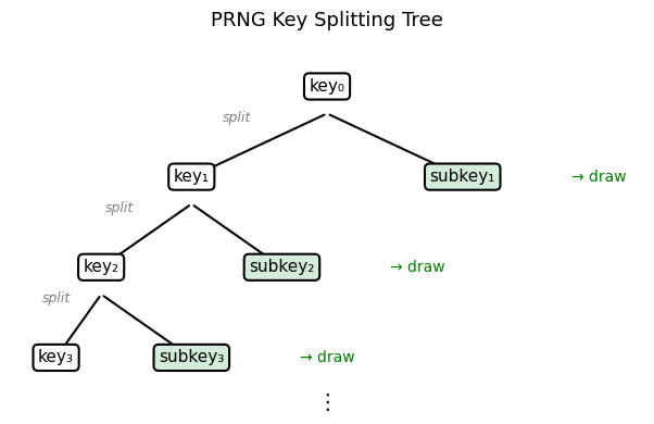
To produce a (quasi-) independent draw, one option is to “split” the existing key:
key, subkey = jax.random.split(key)
jax.random.normal(key, (3, 3))
Array([[ 1.24104247,  0.12018902, -2.23990047],
       [ 0.70507261, -0.85702845, -1.24582014],
       [ 0.38454486,  1.32117717,  0.56866901]], dtype=float64)
jax.random.normal(subkey, (3, 3))
Array([[ 0.07627173, -1.30349831,  0.86524323],
       [-0.75550773,  0.63958052,  0.47052126],
       [-1.72866044, -1.14696564, -1.23328892]], dtype=float64)
The following diagram illustrates how split produces a tree of keys from a
single root, with each key generating independent random draws.
This syntax will seem unusual for a NumPy or Matlab user — but will make more sense when we get to parallel programming.
The function below produces k (quasi-) independent random n x n matrices using split.
def gen_random_matrices(
        key,   # JAX key for random numbers
        n=2,   # Matrices will be n x n
        k=3    # Number of matrices to generate
    ):
    matrices = []
    for _ in range(k):
        key, subkey = jax.random.split(key)
        A = jax.random.uniform(subkey, (n, n))
        matrices.append(A)
    return matrices
seed = 42
key = jax.random.key(seed)
gen_random_matrices(key)
[Array([[0.74211901, 0.54715578],
        [0.05988742, 0.32206803]], dtype=float64),
 Array([[0.65877976, 0.57087415],
        [0.97301903, 0.10138266]], dtype=float64),
 Array([[0.68745522, 0.25974132],
        [0.06595873, 0.83589118]], dtype=float64)]
This function is pure
Deterministic: same inputs, same output
No side effects: no hidden state is modified
14.3.3. Benefits#
As mentioned above, this explicitness is valuable:
Reproducibility: Easy to reproduce results by reusing keys
Parallelization: Control what happens on separate threads
Debugging: No hidden state makes code easier to test
JIT compatibility: The compiler can optimize pure functions more aggressively
14.4. JIT Compilation#
The JAX just-in-time (JIT) compiler accelerates execution by generating efficient machine code that varies with both task size and hardware.
We saw the power of JAX’s JIT compiler combined with parallel hardware when we
above, when we applied cos to a large array.
Here we study JIT compilation for more complex functions
14.4.1. With NumPy#
We’ll try first with NumPy, using
def f(x):
    y = np.cos(2 * x**2) + np.sqrt(np.abs(x)) + 2 * np.sin(x**4) - x**2
    return y
Let’s run with large x
n = 50_000_000
x = np.linspace(0, 10, n)
with qe.Timer():
    # Time NumPy code
    y = f(x)
2.4155 seconds elapsed
Eager execution model
Each operation is executed immediately as it is encountered, materializing its result before the next operation begins.
Disadvantages
Minimal parallelization
Heavy memory footprint — produces many intermediate arrays
Lots of memory read/write
14.4.2. With JAX#
As a first pass, we replace np with jnp throughout:
def f(x):
    y = jnp.cos(2 * x**2) + jnp.sqrt(jnp.abs(x)) + 2 * jnp.sin(x**4) - x**2
    return y


x = jnp.linspace(0, 10, n)
Now let’s time it.
with qe.Timer():
    # First call
    y = f(x)
    # Hold interpreter
    jax.block_until_ready(y);
0.4920 seconds elapsed
with qe.Timer():
    # Second call
    y = f(x)
    # Hold interpreter
    jax.block_until_ready(y);
0.1026 seconds elapsed
The outcome is similar to the cos example — JAX is faster, especially on the
second run after JIT compilation.
This is because the individual array operations are parallelized on the GPU
But we are still using eager execution
lots of memory due to intermediate arrays
lots of memory read/writes
Also, many separate kernels launched on the GPU
14.4.3. Compiling the Whole Function#
Fortunately, with JAX, we have another trick up our sleeve — we can JIT-compile the entire function, not just individual operations.
The compiler fuses all array operations into a single optimized kernel
Let’s try this with the function f:
f_jax = jax.jit(f)
with qe.Timer():
    # First run
    y = f_jax(x)
    # Hold interpreter
    jax.block_until_ready(y);
0.1718 seconds elapsed
with qe.Timer():
    # Second run
    y = f_jax(x)
    # Hold interpreter
    jax.block_until_ready(y);
0.0525 seconds elapsed
The runtime has improved again — now because we fused all the operations
Aggressive optimization based on entire computational sequence
Eliminates multiple calls to the hardware accelerator
The memory footprint is also much lower — no creation of intermediate arrays
Incidentally, a more common syntax when targeting a function for the JIT compiler is
@jax.jit
def f(x):
    pass # put function body here
14.4.4. How JIT compilation works#
When we apply jax.jit to a function, JAX traces it: instead of executing
the operations immediately, it records the sequence of operations as a
computational graph and hands that graph to the
XLA compiler.
XLA then fuses and optimizes the operations into a single compiled kernel tailored to the available hardware (CPU, GPU, or TPU).
The first call to a JIT-compiled function incurs compilation overhead, but subsequent calls with the same input shapes and types reuse the cached compiled code and run at full speed.
14.4.5. Compiling non-pure functions#
While JAX will not usually throw errors when compiling impure functions, execution becomes unpredictable!
Here’s an illustration of this fact:
a = 1  # global

@jax.jit
def f(x):
    return a + x
x = jnp.ones(2)
f(x)
Array([2., 2.], dtype=float64)
In the code above, the global value a=1 is fused into the jitted function.
Even if we change a, the output of f will not be affected — as long as the same compiled version is called.
a = 42
f(x)
Array([2., 2.], dtype=float64)
Changing the dimension of the input triggers a fresh compilation of the function, at which time the change in the value of a takes effect:
x = jnp.ones(3)
f(x)
Array([43., 43., 43.], dtype=float64)
Moral of the story: write pure functions when using JAX!
14.5. Vectorization with vmap#
Another powerful JAX transformation is jax.vmap, which automatically
vectorizes a function written for a single input so that it operates over
batches.
This avoids the need to manually write vectorized code or use explicit loops.
14.5.1. A simple example#
Suppose we have a function that computes the difference between mean and median for an array of numbers.
def mm_diff(x):
    return jnp.mean(x) - jnp.median(x)
We can apply it to a single vector:
x = jnp.array([1.0, 2.0, 5.0])
mm_diff(x)
Array(0.66666667, dtype=float64)
Now suppose we have a matrix and want to compute these statistics for each row.
Without vmap, we’d need an explicit loop:
X = jnp.array([[1.0, 2.0, 5.0],
               [4.0, 5.0, 6.0],
               [1.0, 8.0, 9.0]])

for row in X:
    print(mm_diff(row))
0.6666666666666665
0.0
-2.0
However, Python loops are slow and cannot be efficiently compiled or parallelized by JAX.
With vmap, we can avoid loops and keep the computation on the accelerator:
batch_mm_diff = jax.vmap(mm_diff)    # Create a new "vectorized" version
batch_mm_diff(X)                     # Apply to each row of X
Array([ 0.66666667, 0. , -2. ], dtype=float64)
14.5.2. Combining transformations#
One of JAX’s strengths is that transformations compose naturally.
For example, we can JIT-compile a vectorized function:
fast_batch_mm_diff = jax.jit(jax.vmap(mm_diff))
fast_batch_mm_diff(X)
Array([ 0.66666667, 0. , -2. ], dtype=float64)
This composition of jit, vmap, and (as we’ll see next) grad is central to
JAX’s design and makes it especially powerful for scientific computing and
machine learning.
14.6. Automatic differentiation: a preview#
JAX can use automatic differentiation to compute gradients.
This can be extremely useful for optimization and solving nonlinear systems.
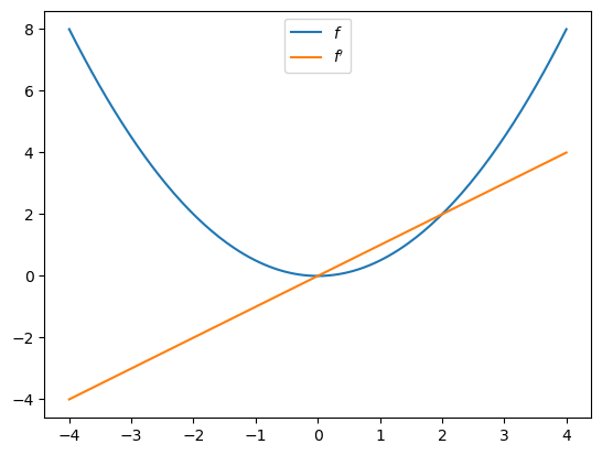
Here’s a simple illustration involving the function \(f(x) = x^2 / 2\):
def f(x):
    return (x**2) / 2

f_prime = jax.grad(f)
f_prime(10.0)
Array(10., dtype=float64, weak_type=True)
Let’s plot the function and derivative, noting that \(f'(x) = x\).
fig, ax = plt.subplots()
x_grid = jnp.linspace(-4, 4, 200)
ax.plot(x_grid, f(x_grid), label="$f$")
ax.plot(x_grid, [f_prime(x) for x in x_grid], label="$f'$")
ax.legend(loc='upper center')
plt.show()
Automatic differentiation is a deep topic with many applications in economics and finance. We provide a more thorough treatment in our lecture on autodiff.
14.7. Exercises#
Exercise 14.1
In the Exercise section of our lecture on Numba, we used Monte Carlo to price a European call option.
The code was accelerated by Numba-based multithreading.
Try writing a version of this operation for JAX, using all the same parameters.
Solution
Here is one solution:
M = 10_000_000

n, β, K = 20, 0.99, 100
μ, ρ, ν, S0, h0 = 0.0001, 0.1, 0.001, 10, 0

@jax.jit
def compute_call_price_jax(β=β,
                           μ=μ,
                           S0=S0,
                           h0=h0,
                           K=K,
                           n=n,
                           ρ=ρ,
                           ν=ν,
                           M=M,
                           key=jax.random.key(1)):

    s = jnp.full(M, np.log(S0))
    h = jnp.full(M, h0)

    def update(i, loop_state):
        s, h, key = loop_state
        key, subkey = jax.random.split(key)
        Z = jax.random.normal(subkey, (2, M))
        s = s + μ + jnp.exp(h) * Z[0, :]
        h = ρ * h + ν * Z[1, :]
        new_loop_state = s, h, key
        return new_loop_state

    initial_loop_state = s, h, key
    final_loop_state = jax.lax.fori_loop(0, n, update, initial_loop_state)
    s, h, key = final_loop_state

    expectation = jnp.mean(jnp.maximum(jnp.exp(s) - K, 0))

    return β**n * expectation
Note
We use jax.lax.fori_loop instead of a Python for loop.
This allows JAX to compile the loop efficiently without unrolling it,
which significantly reduces compilation time for large arrays.
Let’s run it once to compile it:
with qe.Timer():
    compute_call_price_jax().block_until_ready()
1.8637 seconds elapsed
And now let’s time it:
with qe.Timer():
    compute_call_price_jax().block_until_ready()
0.4771 seconds elapsed