1. About These Lectures#
“Python has gotten sufficiently weapons grade that we don’t descend into R anymore. Sorry, R people. I used to be one of you but we no longer descend into R.” – Chris Wiggins
1.1. Overview#
This lecture series will teach you to use Python for scientific computing, with a focus on economics and finance.
The series is aimed at Python novices, although experienced users will also find useful content in later lectures.
In this lecture we will
introduce Python,
showcase some of its abilities,
explain why Python is our favorite language for scientific computing, and
point you to the next steps.
You do not need to understand everything you see in this lecture – we will work through the details slowly later in the lecture series.
1.1.1. Can’t I Just Use LLMs?#
No!
Of course it’s tempting to think that in the age of AI we don’t need to learn how to code.
And yes, we like to be lazy too sometimes.
In addition, we agree that AIs are outstanding productivity tools for coders.
But AIs cannot reliably solve new problems that they haven’t seen before.
You will need to be the architect and the supervisor – and for these tasks you need to be able to read, write, and understand computer code.
Having said that, a good LLM is a useful companion for these lectures – try copy-pasting some code from this series and asking for an explanation.
1.1.2. Isn’t MATLAB Better?#
No, no, and one hundred times no.
Nirvana was great (and Soundgarden was better) but it’s time to move on from the ’90s.
For most modern problems, Python’s scientific libraries are now far in advance of MATLAB’s capabilities.
This is particularly the case in fast-growing fields such as deep learning and reinforcement learning.
Moreover, all major LLMs are more proficient at writing Python code than MATLAB code.
We will discuss relative merits of Python’s libraries throughout this lecture series, as well as in our later series on JAX.
1.2. Introducing Python#
Python is a general-purpose programming language conceived in 1989 by Guido van Rossum.
Python is free and open source, with development coordinated through the Python Software Foundation.
This is important because it
saves us money,
means that Python is controlled by the community of users rather than a for-profit corporation, and
encourages reproducibility and open science.
1.2.1. Common Uses#
Python is a general-purpose language used in almost all application domains, including
AI and computer science
other scientific computing
communication
web development
CGI and graphical user interfaces
game development
resource planning
multimedia
etc.
It is used and supported extensively by large tech firms including
1.2.2. Relative Popularity#
Python is one of the most – if not the most – popular programming languages.
Python libraries like pandas and Polars are replacing familiar tools like Excel and VBA as an essential skill in the fields of finance and banking.
Moreover, Python is extremely popular within the scientific community – especially those connected to AI
For example, the following chart from Stack Overflow Trends shows how the popularity of a single Python deep learning library (PyTorch) has grown over the last few years.
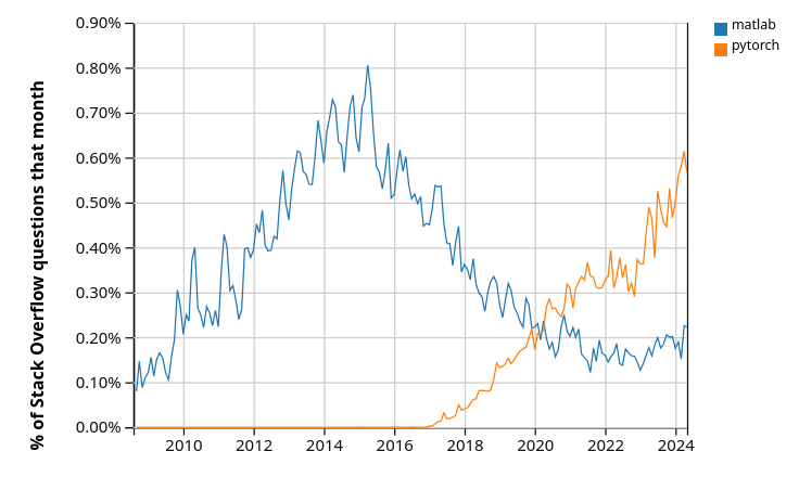
Pytorch is just one of several Python libraries for deep learning and AI.
1.2.3. Features#
Python is a high-level language, which means it is relatively easy to read, write and debug.
It has a relatively small core language that is easy to learn.
This core is supported by many libraries, which can be studied as required.
Python is flexible and pragmatic, supporting multiple programming styles (procedural, object-oriented, functional, etc.).
1.2.4. Syntax and Design#
One reason for Python’s popularity is its simple and elegant design.
To get a feeling for this, let’s look at an example.
The code below is written in Java rather than Python.
You do not need to read and understand this code!
import java.io.BufferedReader;
import java.io.FileReader;
import java.io.IOException;

public class CSVReader {
    public static void main(String[] args) {
        String filePath = "data.csv";
        String line;
        String splitBy = ",";
        int columnIndex = 1;
        double sum = 0;
        int count = 0;

        try (BufferedReader br = new BufferedReader(new FileReader(filePath))) {
            while ((line = br.readLine()) != null) {
                String[] values = line.split(splitBy);
                if (values.length > columnIndex) {
                    try {
                        double value = Double.parseDouble(
                            values[columnIndex]
                        );
                        sum += value;
                        count++;
                    } catch (NumberFormatException e) {
                        System.out.println(
                            "Skipping non-numeric value: " +
                            values[columnIndex]
                        );
                    }
                }
            }
        } catch (IOException e) {
            e.printStackTrace();
        }

        if (count > 0) {
            double average = sum / count;
            System.out.println(
                "Average of the second column: " + average
            );
        } else {
            System.out.println(
                "No valid numeric data found in the second column."
            );
        }
    }
}
This Java code opens an imaginary file called data.csv and computes the mean
of the values in the second column.
Here’s Python code that does the same thing.
Even if you don’t yet know Python, you can see that the code is far simpler and easier to read.
import csv

total, count = 0, 0
with open('data.csv', mode='r') as file:
    reader = csv.reader(file)
    for row in reader:
        try:
            total += float(row[1])
            count += 1
        except (ValueError, IndexError):
            pass
print(f"Average: {total / count if count else 'No valid data'}")
1.2.5. The AI Connection#
AI is in the process of taking over many tasks currently performed by humans, just as other forms of machinery have done over the past few centuries.
Moreover, Python is playing a huge role in the advance of AI and machine learning.
This means that tech firms are pouring money into development of extremely powerful Python libraries.
Even if you don’t plan to work on AI and machine learning, you can benefit from learning to use some of these libraries for your own projects in economics, finance and other fields of science.
These lectures will explain how.
1.3. Scientific Programming with Python#
We have already discussed the importance of Python for AI, machine learning and data science
Python is also one of the dominant players in
astronomy
chemistry
computational biology
meteorology
natural language processing
etc.
Use of Python is also rising in economics, finance, and adjacent fields like operations research – which were previously dominated by MATLAB / Excel / STATA / C / Fortran.
This section briefly showcases some examples of Python for general scientific programming.
1.3.1. NumPy#
One of the most important parts of scientific computing is working with data.
Data is often stored in matrices, vectors and arrays.
We can create a simple array of numbers with pure Python as follows:
a = [-3.14, 0, 3.14]                    # A Python list
a
[-3.14, 0, 3.14]
This array is very small so it’s fine to work with pure Python.
But when we want to work with larger arrays in real programs we need more efficiency and more tools.
For this we need to use libraries for working with arrays.
For Python, the most important matrix and array processing library is NumPy library.
For example, let’s build a NumPy array with 100 elements
import numpy as np                     # Load the library

a = np.linspace(-np.pi, np.pi, 100)    # Create even grid from -π to π
a
array([-3.14159265, -3.07812614, -3.01465962, -2.9511931 , -2.88772658,
       -2.82426006, -2.76079354, -2.69732703, -2.63386051, -2.57039399,
       -2.50692747, -2.44346095, -2.37999443, -2.31652792, -2.2530614 ,
       -2.18959488, -2.12612836, -2.06266184, -1.99919533, -1.93572881,
       -1.87226229, -1.80879577, -1.74532925, -1.68186273, -1.61839622,
       -1.5549297 , -1.49146318, -1.42799666, -1.36453014, -1.30106362,
       -1.23759711, -1.17413059, -1.11066407, -1.04719755, -0.98373103,
       -0.92026451, -0.856798  , -0.79333148, -0.72986496, -0.66639844,
       -0.60293192, -0.53946541, -0.47599889, -0.41253237, -0.34906585,
       -0.28559933, -0.22213281, -0.1586663 , -0.09519978, -0.03173326,
        0.03173326,  0.09519978,  0.1586663 ,  0.22213281,  0.28559933,
        0.34906585,  0.41253237,  0.47599889,  0.53946541,  0.60293192,
        0.66639844,  0.72986496,  0.79333148,  0.856798  ,  0.92026451,
        0.98373103,  1.04719755,  1.11066407,  1.17413059,  1.23759711,
        1.30106362,  1.36453014,  1.42799666,  1.49146318,  1.5549297 ,
        1.61839622,  1.68186273,  1.74532925,  1.80879577,  1.87226229,
        1.93572881,  1.99919533,  2.06266184,  2.12612836,  2.18959488,
        2.2530614 ,  2.31652792,  2.37999443,  2.44346095,  2.50692747,
        2.57039399,  2.63386051,  2.69732703,  2.76079354,  2.82426006,
        2.88772658,  2.9511931 ,  3.01465962,  3.07812614,  3.14159265])
Now let’s transform this array by applying functions to it.
b = np.cos(a)                          # Apply cosine to each element of a
c = np.sin(a)                          # Apply sin to each element of a
Now we can easily take the inner product of b and c.
b @ c
np.float64(2.706168622523819e-16)
We can also do many other tasks, like
compute the mean and variance of arrays
build matrices and solve linear systems
generate random arrays for simulation, etc.
We will discuss the details later in the lecture series, where we cover NumPy in depth.
1.3.2. NumPy Alternatives#
While NumPy is still the king of array processing in Python, there are now important competitors.
Libraries such as JAX, Pytorch, and CuPy also have built in array types and array operations that can be very fast and efficient.
In fact these libraries are better at exploiting parallelization and fast hardware, as we’ll explain later in this series.
However, you should still learn NumPy first because
NumPy is simpler and provides a strong foundation, and
libraries like JAX directly extend NumPy functionality and hence are easier to learn when you already know NumPy.
This lecture series will provide you with extensive background in NumPy.
1.3.3. SciPy#
The SciPy library is built on top of NumPy and provides additional functionality.
For example, let’s calculate \(\int_{-2}^2 \phi(z) dz\) where \(\phi\) is the standard normal density.
from scipy.stats import norm
from scipy.integrate import quad

ϕ = norm()
value, error = quad(ϕ.pdf, -2, 2)  # Integrate using Gaussian quadrature
value
0.9544997361036417
SciPy includes many of the standard routines used in
See them all here.
Later we’ll discuss SciPy in more detail.
1.3.4. Graphics#
A major strength of Python is data visualization.
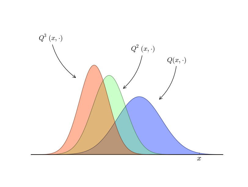
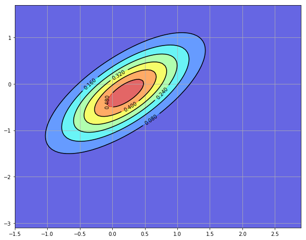
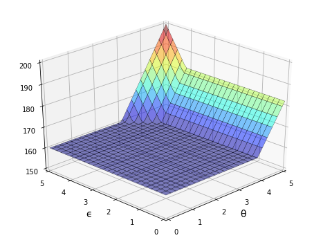
The most popular and comprehensive Python library for creating figures and graphs is Matplotlib, with functionality including
plots, histograms, contour images, 3D graphs, bar charts etc.
output in many formats (PDF, PNG, EPS, etc.)
LaTeX integration
Example 2D plot with embedded LaTeX annotations
Example contour plot
Example 3D plot
More examples can be found in the Matplotlib thumbnail gallery.
Other graphics libraries include
You can visit the Python Graph Gallery for more example plots drawn using a variety of libraries.
1.3.5. Networks and Graphs#
The study of networks is becoming an important part of scientific work in economics, finance and other fields.
For example, we are interesting in studying
production networks
networks of banks and financial institutions
friendship and social networks
etc.
Python has many libraries for studying networks and graphs.
One well-known example is NetworkX.
Its features include, among many other things:
standard graph algorithms for analyzing networks
plotting routines
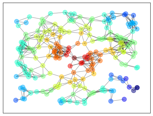
Here’s some example code that generates and plots a random graph, with node color determined by the shortest path length from a central node.
import networkx as nx
import matplotlib.pyplot as plt
np.random.seed(1234)

# Generate a random graph
p = dict((i, (np.random.uniform(0, 1), np.random.uniform(0, 1)))
         for i in range(200))
g = nx.random_geometric_graph(200, 0.12, pos=p)
pos = nx.get_node_attributes(g, 'pos')

# Find node nearest the center point (0.5, 0.5)
dists = [(x - 0.5)**2 + (y - 0.5)**2 for x, y in list(pos.values())]
ncenter = np.argmin(dists)

# Plot graph, coloring by path length from central node
p = nx.single_source_shortest_path_length(g, ncenter)
plt.figure()
nx.draw_networkx_edges(g, pos, alpha=0.4)
nx.draw_networkx_nodes(g,
                       pos,
                       nodelist=list(p.keys()),
                       node_size=120, alpha=0.5,
                       node_color=list(p.values()),
                       cmap=plt.cm.jet_r)
plt.show()
1.3.6. Other Scientific Libraries#
As discussed above, there are literally thousands of scientific libraries for Python.
Some are small and do very specific tasks.
Others are huge in terms of lines of code and investment from coders and tech firms.
Here’s a short list of some important scientific libraries for Python not mentioned above.
SymPy for symbolic algebra, including limits, derivatives and integrals
statsmodels for statistical routines
scikit-learn for machine learning
Keras for machine learning
GeoPandas for spatial data analysis
Dask for parallelization
Numba for making Python run at the same speed as native machine code
CVXPY for convex optimization
scikit-image and OpenCV for processing and analyzing image data
BeautifulSoup for extracting data from HTML and XML files
In this lecture series we will learn how to use many of these libraries for scientific computing tasks in economics and finance.