15. NumPy vs Numba vs JAX#
In the preceding lectures, we’ve discussed three core libraries for scientific and numerical computing:
Which one should we use in any given situation?
This lecture addresses that question, at least partially, by discussing some use cases.
Before getting started, we note that the first two are a natural pair: NumPy and Numba play well together.
JAX, on the other hand, stands alone.
When considering each approach, we will consider not just efficiency and memory footprint but also clarity and ease of use.
In addition to what’s in Anaconda, this lecture will need the following libraries:
!pip install quantecon jax
GPU
This lecture was built using a machine with access to a GPU — although it will also run without one.
Google Colab has a free tier with GPUs that you can access as follows:
Click on the “play” icon top right
Select Colab
Set the runtime environment to include a GPU
We will use the following imports.
from functools import partial

import numpy as np
import numba
import quantecon as qe
import matplotlib.pyplot as plt
from mpl_toolkits.mplot3d.axes3d import Axes3D
from matplotlib import cm
import jax
import jax.numpy as jnp
from jax import lax
15.1. Vectorized operations#
Some operations can be perfectly vectorized — all loops are easily eliminated and numerical operations are reduced to calculations on arrays.
In this case, which approach is best?
15.1.1. Problem Statement#
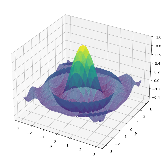
Consider the problem of maximizing a function \(f\) of two variables \((x,y)\) over the square \([-a, a] \times [-a, a]\).
For \(f\) and \(a\) let’s choose
Here’s a plot of \(f\)
def f(x, y):
    return np.cos(x**2 + y**2) / (1 + x**2 + y**2)

xgrid = np.linspace(-3, 3, 50)
ygrid = xgrid
x, y = np.meshgrid(xgrid, ygrid)

fig = plt.figure(figsize=(10, 8))
ax = fig.add_subplot(111, projection='3d')
ax.plot_surface(x,
                y,
                f(x, y),
                rstride=2, cstride=2,
                cmap=cm.viridis,
                alpha=0.7,
                linewidth=0.25)
ax.set_zlim(-0.5, 1.0)
ax.set_xlabel('$x$', fontsize=14)
ax.set_ylabel('$y$', fontsize=14)
plt.show()
For the sake of this exercise, we’re going to use brute force for the maximization.
Evaluate \(f\) for all \((x,y)\) in a grid on the square.
Return the maximum of observed values.
Just to illustrate the idea, here’s a non-vectorized version that uses Python loops.
grid = np.linspace(-3, 3, 50)
m = -np.inf
for x in grid:
    for y in grid:
        z = f(x, y)
        m = max(m, z)
15.1.2. NumPy vectorization#
Let’s switch to NumPy and use a larger grid
grid = np.linspace(-3, 3, 3_000) # Large grid
As a first pass of vectorization we might try something like this
# Large grid
z = np.max(f(grid, grid))    # This is wrong!
The problem here is that f(grid, grid) doesn’t obey the nested loop.
In terms of the figure above, it only computes the values of f along the
diagonal.
To trick NumPy into calculating f(x,y) on every x,y pair, we need to use np.meshgrid.
Here we use np.meshgrid to create two-dimensional input grids x and y
such that f(x, y) generates all evaluations on the product grid.
# Large grid
grid = np.linspace(-3, 3, 3_000)

x_mesh, y_mesh = np.meshgrid(grid, grid)      # MATLAB style meshgrid

with qe.Timer():
    z_max_numpy = np.max(f(x_mesh, y_mesh))   # This works
0.2551 seconds elapsed
In the vectorized version, all the looping takes place in compiled code.
The use of meshgrid allows us to replicate the nested for loop.
The output should be close to one:
print(f"NumPy result: {z_max_numpy:.6f}")
NumPy result: 0.999998
15.1.3. Memory Issues#
So we have the right solution in reasonable time — but memory usage is huge.
While the flat arrays are low-memory
grid.nbytes
24000
the mesh grids are two-dimensional and hence very memory intensive
x_mesh.nbytes + y_mesh.nbytes
144000000
Moreover, NumPy’s eager execution creates many intermediate arrays of the same size!
This kind of memory usage can be a big problem in actual research calculations.
15.1.4. A Comparison with Numba#
Let’s see if we can achieve better performance using Numba with a simple loop.
@numba.jit
def compute_max_numba(grid):
    m = -np.inf
    for x in grid:
        for y in grid:
            z = np.cos(x**2 + y**2) / (1 + x**2 + y**2)
            m = max(m, z)
    return m
Let’s test it:
grid = np.linspace(-3, 3, 3_000)

with qe.Timer():
    # First run
    z_max_numba = compute_max_numba(grid)
0.2780 seconds elapsed
Let’s run again to eliminate compile time.
with qe.Timer():
    # Second run
    compute_max_numba(grid)
0.1511 seconds elapsed
Notice how we are using almost no memory — we just need the one-dimensional grid
Moreover, execution speed is good.
On most machines, the Numba version will be somewhat faster than NumPy.
The reason is efficient machine code plus less memory read-write.
15.1.5. Parallelized Numba#
Now let’s try parallelization with Numba using prange:
@numba.jit(parallel=True)
def compute_max_numba_parallel(grid):
    n = len(grid)
    m = -np.inf
    for i in numba.prange(n):
        for j in range(n):
            x = grid[i]
            y = grid[j]
            z = np.cos(x**2 + y**2) / (1 + x**2 + y**2)
            m = max(m, z)
    return m
Here’s a warm up run and test.
with qe.Timer():
    # First run
    z_max_parallel = compute_max_numba_parallel(grid)
0.6309 seconds elapsed
Here’s the timing for the pre-compiled version.
with qe.Timer():
    # Second run
    compute_max_numba_parallel(grid)
0.0286 seconds elapsed
If you have multiple cores, you should see benefits from parallelization here.
Let’s make sure we’re still getting the right result (close to one):
print(f"Numba result: {z_max_parallel:.6f}")
Numba result: 0.999998
For powerful machines and larger grid sizes, parallelization can generate useful speed gains, even on the CPU.
15.1.6. Vectorized code with JAX#
Let’s try replicating the NumPy vectorized approach with JAX.
Let’s start with the function, which switches np to jnp and adds jax.jit
@jax.jit
def f(x, y):
    return jnp.cos(x**2 + y**2) / (1 + x**2 + y**2)
We use the NumPy style meshgrid approach:
grid = jnp.linspace(-3, 3, 3_000)
x_mesh, y_mesh = jnp.meshgrid(grid, grid)
Now let’s run and time
with qe.Timer():
    # First run
    z_max = jnp.max(f(x_mesh, y_mesh))
    # Hold interpreter
    z_max.block_until_ready()

print(f"Plain vanilla JAX result: {z_max:.6f}")
0.2434 seconds elapsed
Plain vanilla JAX result: 0.999998
Let’s run again to eliminate compile time.
with qe.Timer():
    # Second run
    z_max = jnp.max(f(x_mesh, y_mesh))
    # Hold interpreter
    z_max.block_until_ready()
0.0008 seconds elapsed
Once compiled, JAX is significantly faster than NumPy, especially on a GPU.
The compilation overhead is a one-time cost that pays off when the function is called repeatedly.
15.1.7. JAX plus vmap#
Because we used jax.jit above, we avoided creating many intermediate arrays.
But we still create the big arrays z_max, x_mesh, and y_mesh.
Fortunately, we can avoid this by using jax.vmap.
Here’s how we can apply it to our problem.
@jax.jit
def compute_max_vmap(grid):
    # Construct a function that takes the max over all x for given y
    compute_column_max = lambda y: jnp.max(f(grid, y))
    # Vectorize the function so we can call on all y simultaneously
    vectorized_compute_column_max = jax.vmap(compute_column_max)
    # Compute the column max at every row
    column_maxes = vectorized_compute_column_max(grid)
    # Compute the max of the column maxes and return
    return jnp.max(column_maxes)
Note that we never create
the two-dimensional grid
x_meshthe two-dimensional grid
y_meshorthe two-dimensional array
f(x,y)
Like Numba, we just use the flat array grid.
And because everything is under a single @jax.jit, the compiler can fuse
all operations into one optimized kernel.
Let’s try it.
with qe.Timer():
    # First run
    z_max = compute_max_vmap(grid)
    # Hold interpreter
    z_max.block_until_ready()

print(f"JAX vmap result: {z_max:.6f}")
0.2580 seconds elapsed
JAX vmap result: 0.999998
Let’s run it again to eliminate compilation time:
with qe.Timer():
    # Second run
    z_max = compute_max_vmap(grid)
    # Hold interpreter
    z_max.block_until_ready()
0.0003 seconds elapsed
15.1.8. Summary#
In our view, JAX is the winner for vectorized operations.
It dominates NumPy both in terms of speed (via JIT-compilation and parallelization) and memory efficiency (via vmap).
It also dominates Numba when run on the GPU.
Note
Numba can support GPU programming through numba.cuda but then we need to
parallelize by hand. For most cases encountered in economics, econometrics, and finance, it is
far better to hand over to the JAX compiler for efficient parallelization than to
try to hand-code these routines ourselves.
15.2. Sequential operations#
Some operations are inherently sequential – and hence difficult or impossible to vectorize.
In this case NumPy is a poor option and we are left with the choice of Numba or JAX.
To compare these choices, we will revisit the problem of iterating on the quadratic map that we saw in our Numba lecture.
15.2.1. Numba Version#
Here’s the Numba version.
@numba.jit
def qm(x0, n, α=4.0):
    x = np.empty(n+1)
    x[0] = x0
    for t in range(n):
      x[t+1] = α * x[t] * (1 - x[t])
    return x
Let’s generate a time series of length 10,000,000 and time the execution:
n = 10_000_000

with qe.Timer():
    # First run
    x = qm(0.1, n)
0.1598 seconds elapsed
Let’s run it again to eliminate compilation time:
with qe.Timer():
    # Second run
    x = qm(0.1, n)
0.0708 seconds elapsed
Numba handles this sequential operation very efficiently.
15.2.2. JAX Version#
We cannot directly replace numba.jit with jax.jit because JAX arrays are immutable.
But we can still implement this operation
15.2.2.1. First Attempt#
Here’s a workaround using the at[t].set syntax we discussed in the JAX lecture.
We’ll apply a lax.fori_loop, which is a version of a for loop that can be compiled by XLA.
cpu = jax.devices("cpu")[0]

@partial(jax.jit, static_argnames=("n",), device=cpu)
def qm_jax_fori(x0, n, α=4.0):

    x = jnp.empty(n + 1).at[0].set(x0)

    def update(t, x):
        return x.at[t + 1].set(α * x[t] * (1 - x[t]))

    x = lax.fori_loop(0, n, update, x)
    return x
We hold
nstatic because it affects array size and hence JAX wants to specialize on its value in the compiled code.We pin to the CPU via
device=cpubecause this sequential workload consists of many small operations, leaving little opportunity for GPU parallelism.
Important: Although at[t].set appears to create a new array at each step, inside a JIT-compiled function the compiler detects that the old array is no longer needed and performs the update in place!
Let’s time it with the same parameters:
with qe.Timer():
    # First run
    x_jax = qm_jax_fori(0.1, n)
    # Hold interpreter
    x_jax.block_until_ready()
0.1208 seconds elapsed
Let’s run it again to eliminate compilation overhead:
with qe.Timer():
    # Second run
    x_jax = qm_jax_fori(0.1, n)
    # Hold interpreter
    x_jax.block_until_ready()
0.0617 seconds elapsed
JAX is also quite efficient for this sequential operation!
15.2.2.2. Second Attempt#
There’s another way we can implement the loop that uses lax.scan.
This alternative is arguably more in line with JAX’s functional approach — although the syntax is difficult to remember.
@partial(jax.jit, static_argnames=("n",), device=cpu)
def qm_jax_scan(x0, n, α=4.0):
    def update(x, t):
        x_new = α * x * (1 - x)
        return x_new, x_new

    _, x = lax.scan(update, x0, jnp.arange(n))
    return jnp.concatenate([jnp.array([x0]), x])
This code is not easy to read but, in essence, lax.scan repeatedly calls update and accumulates the returns x_new into an array.
Let’s time it with the same parameters:
with qe.Timer():
    # First run
    x_jax = qm_jax_scan(0.1, n)
    # Hold interpreter
    x_jax.block_until_ready()
0.1300 seconds elapsed
Let’s run it again to eliminate compilation overhead:
with qe.Timer():
    # Second run
    x_jax = qm_jax_scan(0.1, n)
    # Hold interpreter
    x_jax.block_until_ready()
0.0699 seconds elapsed
Surprisingly, JAX also delivers strong performance after compilation.
15.2.3. Summary#
While both Numba and JAX deliver strong performance for sequential operations, there are differences in code readability and ease of use.
The Numba version is straightforward and natural to read: we simply allocate an array and fill it element by element using a standard Python loop.
This is exactly how most programmers think about the algorithm.
The JAX versions, on the other hand, require either lax.fori_loop or
lax.scan, both of which are less intuitive than a standard Python loop.
While JAX’s at[t].set syntax does allow element-wise updates, the overall code
remains harder to read than the Numba equivalent.
15.3. Overall recommendations#
Let’s now step back and summarize the trade-offs.
For vectorized operations, JAX is the strongest choice.
It matches or exceeds NumPy in speed, thanks to JIT compilation and efficient parallelization across CPUs and GPUs.
The vmap transformation reduces memory usage and often leads to clearer code
than traditional meshgrid-based vectorization.
In addition, JAX functions are automatically differentiable, as we explore in Adventures with Autodiff.
For sequential operations, Numba has nicer syntax.
The code is natural and readable — just a Python loop with a decorator — and performance is excellent.
JAX can handle sequential problems via lax.fori_loop or lax.scan, but
the syntax is less intuitive.
On the other hand, the JAX versions support automatic differentiation.
That might be of interest if, say, we want to compute sensitivities of a trajectory to model parameters